breed [ sheep a-sheep ] ; sheep subtype of turtlebreed [ wolves wolf ] ; wolf subtype of turtleturtles-own [ energy ] ; add energy attr to W + Spatches-own [ countdown ] ; add countdown attr to grid
to eat-sheep ; wolf procedure let prey one-of sheep-here ; grab a random sheepif prey != nobody [ ask prey [ die ] ; eat itset energy energy + wolf-gain-from-food ; get energy ]end
ask sheep [ moveset energy energy -1 eat-grass death ; sheep die if they run out of energy reproduce-sheep ]ask wolves [ moveset energy energy -1 eat-sheep ; wolves eat a sheep on their patch death ; wolves die if they run out of energy reproduce-wolves ;]ask patches [ grow-grass ]tick
mutable struct PoorSoul <: AbstractAgent id::Int pos::NTuple{2,Float64} vel::NTuple{2,Float64} mass::Float64 days_infected::Int # number of days since is infected status::Symbol # :S, :I or :R β::Float64end
Dynamics
functionelastic_collision!(a, b) v1, v2, x1, x2 = a.vel, b.vel, a.pos, b.poslength(v1) !=2&&error("This works only for 2D") r1 = x1 .- x2; r2 = x2 .- x1 !(dot(r2, v1) >0&&dot(r2, v1) >0) &&returnfalse dx,dv = a.pos .- b.pos, a.vel .- b.vel n =norm(dx)^2 n ==0&&returnfalse# do nothing if at the same pos. a.vel = v1 .- ( dot(v1 .- v2, r1) / n ) .* (r1) b.vel = v2 .- ( dot(v2 .- v1, r2) / n ) .* (r2)returntrueend
Control flow
for (a1, a2) ininteracting_pairs(model, model.radius)transmit!(a1, a2, model.reinfection_probability)elastic_collision!(a1, a2)end
breed [ sheep a-sheep ] ; sheep subtype of turtlebreed [ wolves wolf ] ; wolf subtype of turtleturtles-own [ energy ] ; add energy attr to W + Spatches-own [ countdown ] ; add countdown attr to grid
Dynamics
to eat-sheep ; wolf procedure let prey one-of sheep-here ; grab a random sheepif prey != nobody [ ask prey [ die ] ; eat itset energy energy + wolf-gain-from-food ; get energy ]end
Control flow
ask sheep [ moveset energy energy -1 eat-grass death ; sheep die if they run out of energy reproduce-sheep ]ask wolves [ moveset energy energy -1 eat-sheep ; wolves eat a sheep on their patch death ; wolves die if they run out of energy reproduce-wolves ;]ask patches [ grow-grass ]
I. Challenges with getting engineers into graph rewriting
The syntax of graph rewrite rules has the virtues we want, but:
It is a syntax for atomic changes. Nondeterminism from match and rule choice.
Engineers / modelers need more determinism / coordinated rewriting.
What is a good syntax for talking about the algorithmic application of rewrite rules?1
I. General strategies for control
Unordered rules, but control via constraints / maintain program state ‘in the graph’
Directed graph of rewrite rules
No control of matches
No complex control flow
General program with rewrite primatives
No explicit control of matches
Program language syntax
We want a graphical language for control flow + one which lets us say “use this match”.
Manually, by specifying each component (e.g. V=[2,3], E=[1])
Via automated search + constraints, (e.g. monic=true)
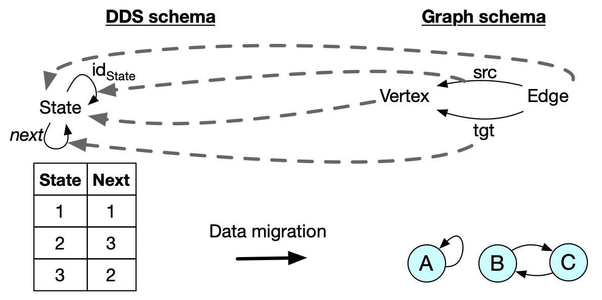
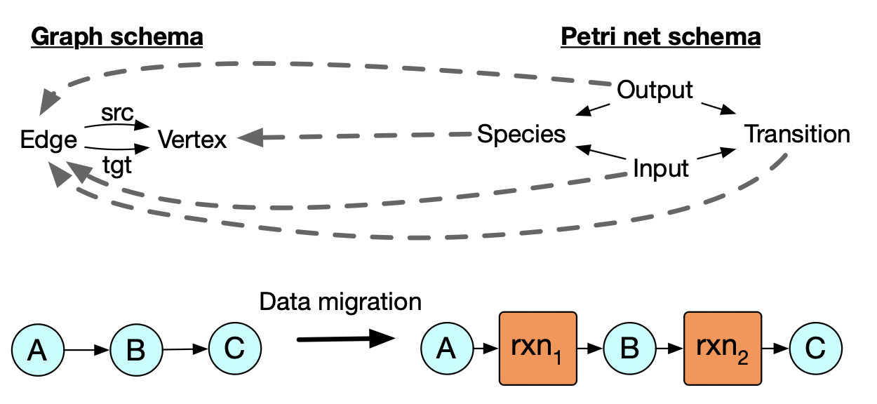
CSet schemas (ACSet schemas)
DDS, Graph, Petri Net (ChemicalRxn)
Data migration:
Functor between schemas presents transformation process on instances
DDS to Graph, Graph to Petri Net
II. AlgebraicRewriting basics
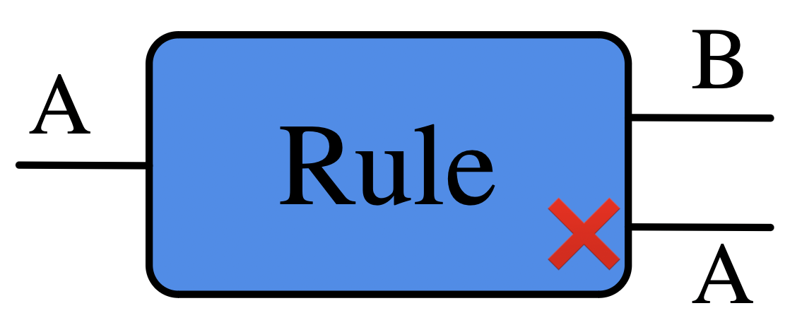
AlgebraicRewriting introduces the Rule data structure:
zero =Graph(0)edge =path_graph(Graph, 2)del_edge =Rule{:SPO}(homomorphism(zero, edge), # L <- Iid(zero); # I -> R monic=true# constraints on the match morphisms ac=[PAC(...), NAC(...)] # feed in morphisms L -> P, L -> N)rewrite(del_edge, G) # result of applying an arbitrary matchL_to_G =homomorphism(edge, G) # pick a specific matchrewrite_match(del_edge, L_to_G) # rewrite with a specific matchres =rewrite_match_maps(del_edge, L_to_G) # return the entire derivation diagram
Attributed \(\mathsf{C}\)-Sets (ACSets) can have concrete attribute values or variables (AttrVars).
We can manipute the concrete variables with custom code
L =@acset WeightedGraph{Float64} begin V=2; E=2; Weight=2; src=[1,1]; tgt=[2,2]; weight=[AttrVar(1), AttrVar(2)] endI =WeightedGraph{Float64}(2)R =@acset WeightedGraph{Float64} begin V=2; E=1; Weight=1; src=1; tgt=2; weight=[AttrVar(1)] endl =homomorphism(I,L; monic=true)r =homomorphism(I,R; monic=true)merge_multiply =Rule(l, r; monic=[:E], expr=Dict(:Weight=>[(w1, w2) -> w1*w2]))
III. Rewrite programs: SMCs
Symmetric monoidal categories are a desirable structure for one’s syntax to have:
Can be graphically depicted
Can serve as the syntax for varying semantics
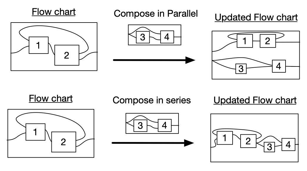
III. Rewrite programs: SMC composition
Symmetric monoidal categories are a desirable structure for one’s syntax to have:
Can be graphically depicted
Can serve as the syntax for varying semantics
Can be composed in parallel or in series
With further traced structure, we can have loops.
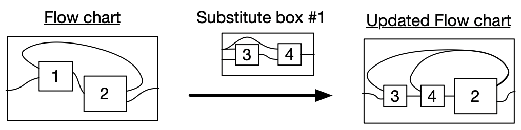
III. Rewrite programs: SMC substitution
Symmetric monoidal categories are a desirable structure for one’s syntax to have:
Can be graphically depicted
Can serve as the syntax for varying semantics
Can be composed in parallel or in series
With further traced structure, we can have loops.
Can be operadically substituted
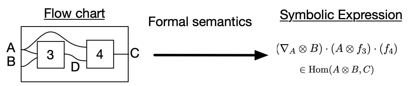
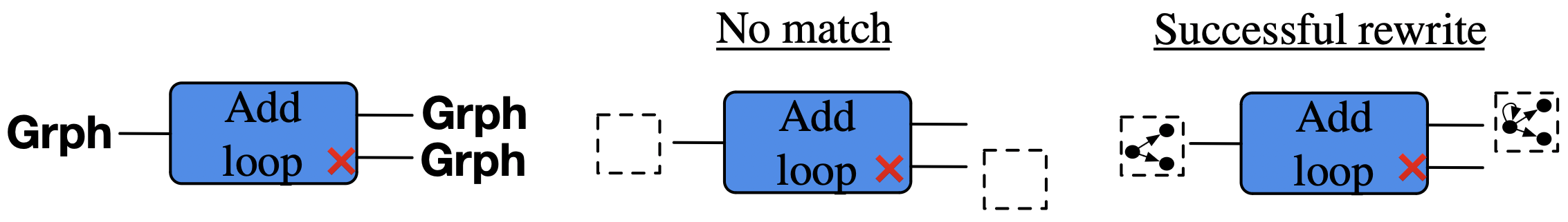
Graphical language of function composition
\(\mathbf{Set_*}\) has the required traced monoidal structure (using coproducts for \(\otimes\)).
Thus we can use this language to talk about composition of functions.
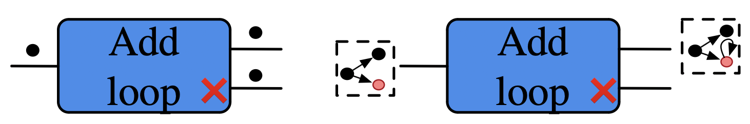
Think of rewrite rule add_loop as a function1\(Grph \rightarrow Grph + Grph\):
Add a loop to a vertex. If none exists, then add a vertex, then give it a loop.
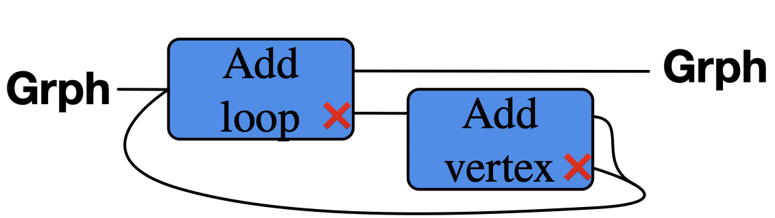
Graphical language of function composition
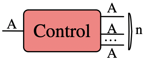
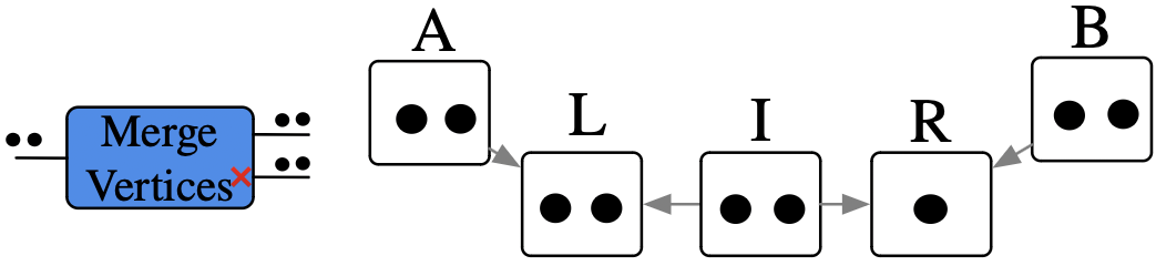
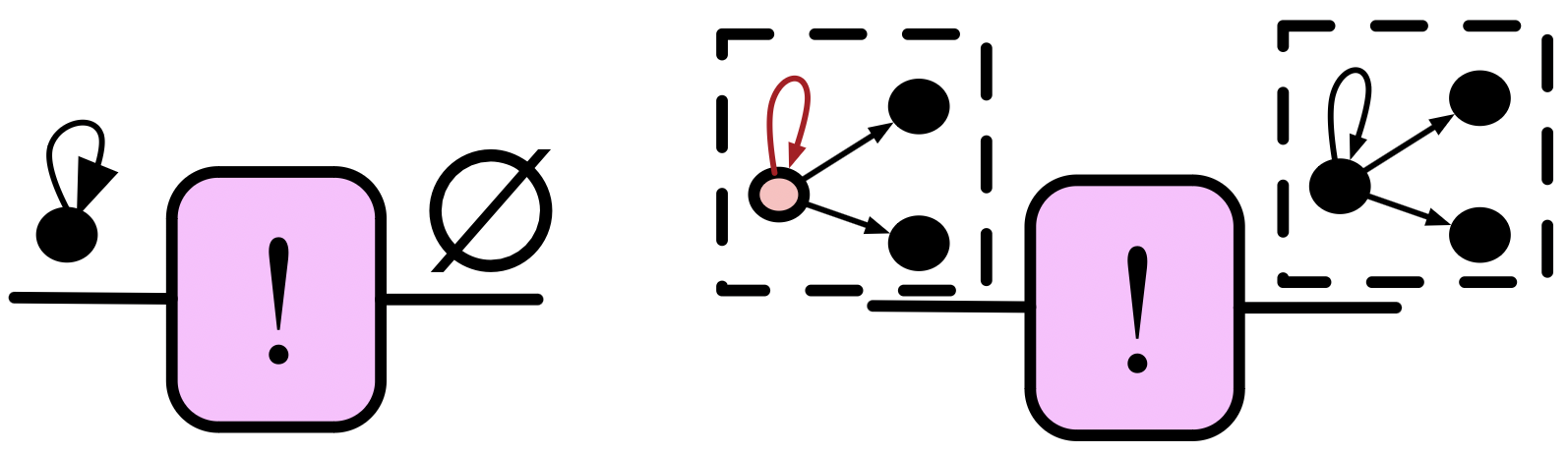
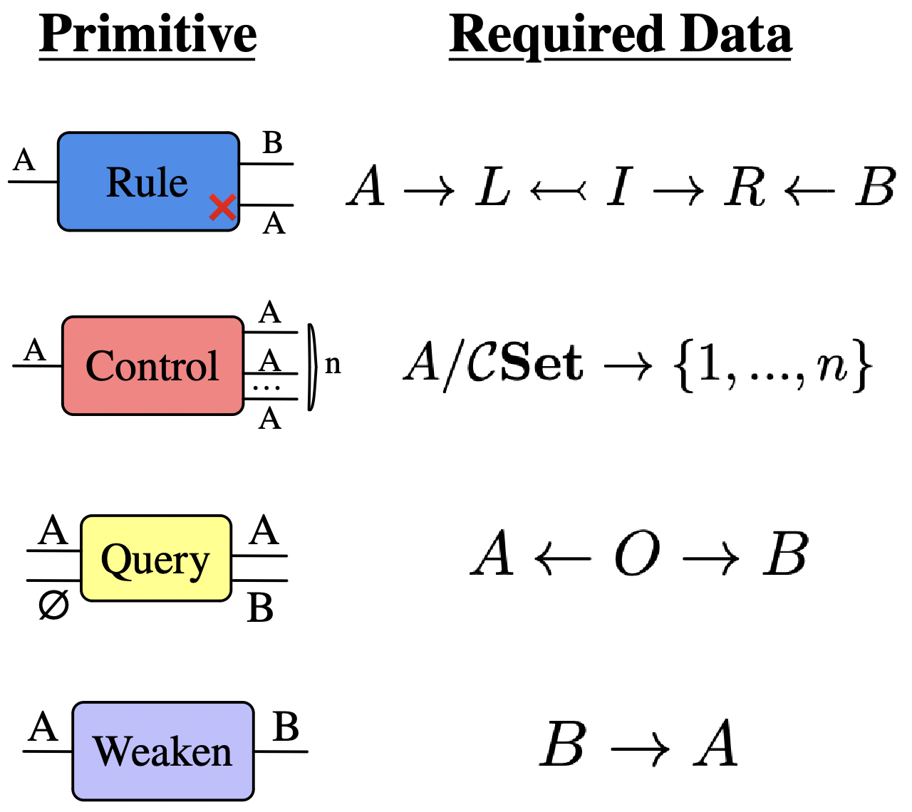
New primitive type of box for control flow:
Can only redirect its input, not modify it
\(A \xrightarrow{f} n \times A\) for \(n \in \mathbb{N}\) such that \(f\cdot \pi_i = id_A\)
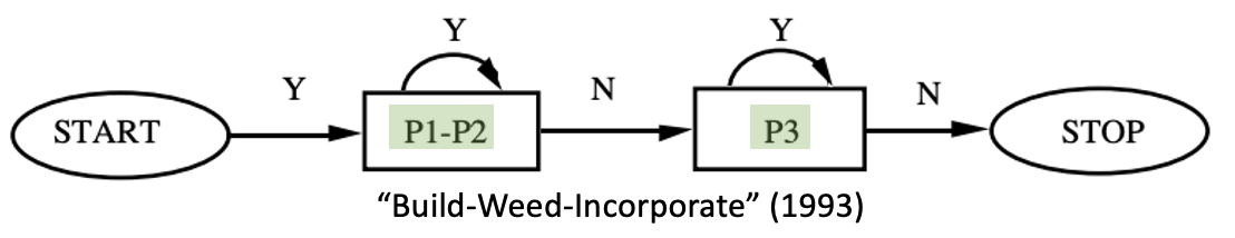
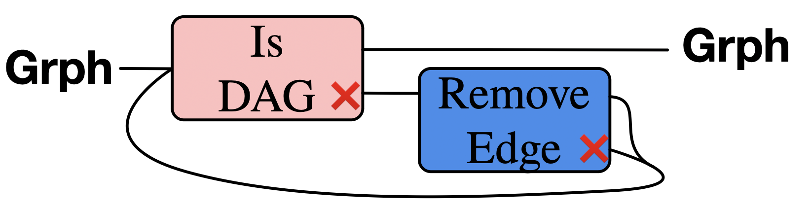
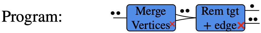
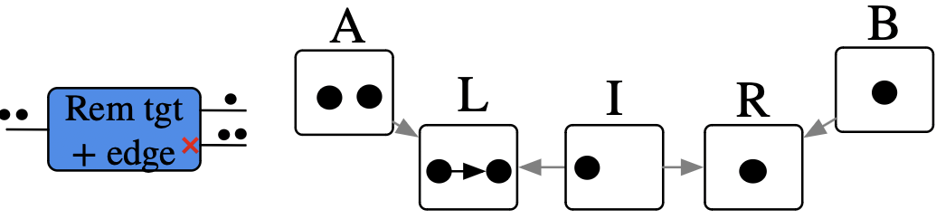
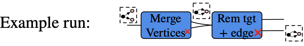
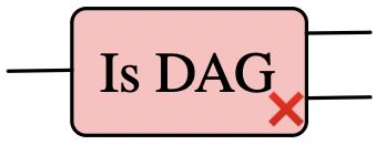
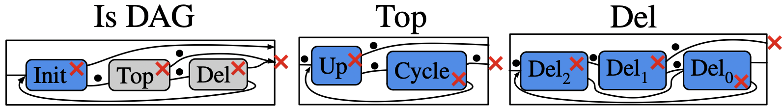
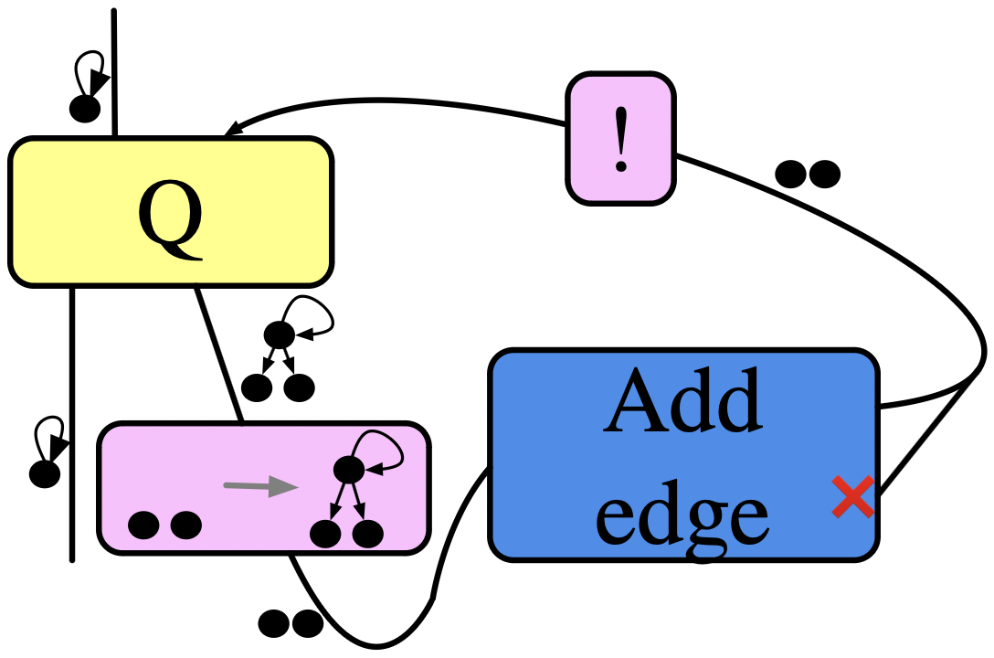
Remove edges, until we have a DAG
Remove an edge, distinguish between cases of empty result or not
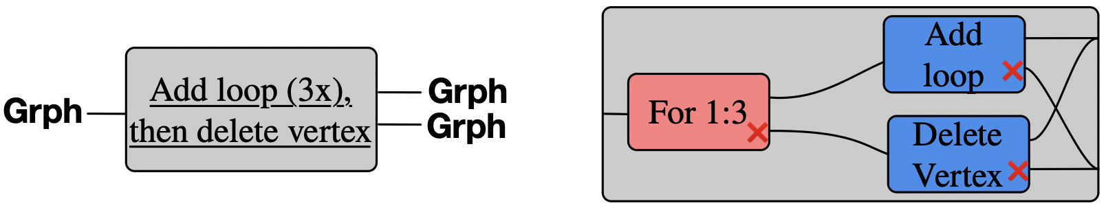
Graphical language of dynamic function composition
Mealy machines (or dynamic functions) seem to form a symmetric monoidal category.1
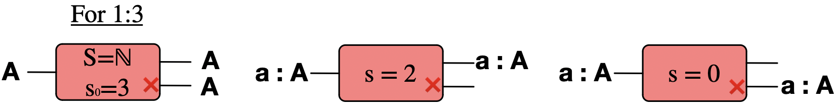
A control flow box which decrements its internal state each time it is entered:
A box which behaves like Add Loop the first three times it is used, then like Delete Vertex:
Control of matches via a notion of ‘agent’
Our wires are labeled with “agent shapes”. These are \(\mathsf{C}\)-Sets.
Set of possible values associated with a wire is the set of morphisms\(A \rightarrow G\) for some \(\mathsf{C}\)-Set \(G\).
Crucial difference between adding a loop to some vertex vs adding a loop to this vertex.
Gradient between two extremes:
determinism (\(A = L\))
nondeterminism (\(A = \varnothing\))
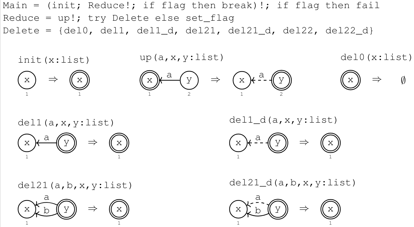
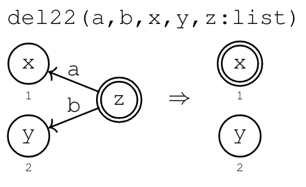
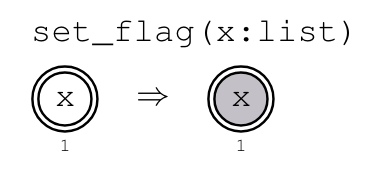
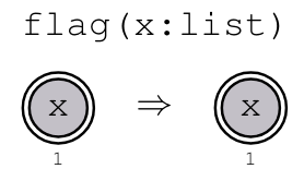
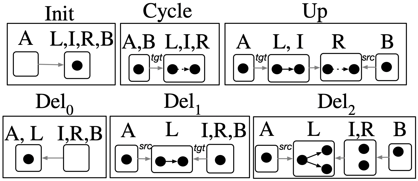
Example of rewriting with control of matches
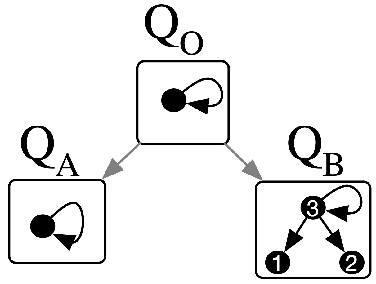
Example: Binary DAGs
Suppose we want to classify binary DAGs1
Example: Binary DAGs
Rewrite program in a category with schema \(\boxed{V \leftleftarrows E \leftarrow Seen}\)
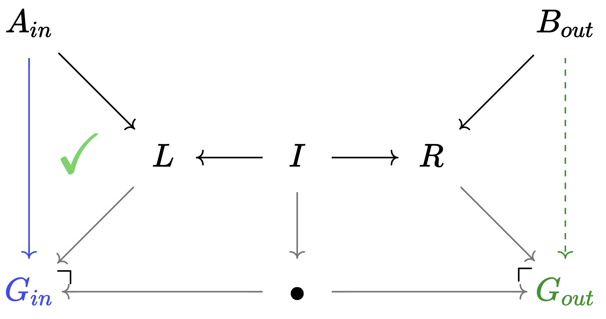
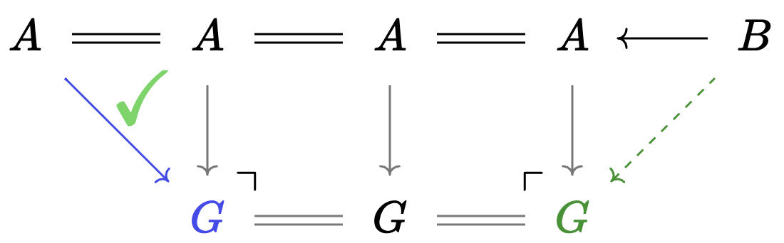
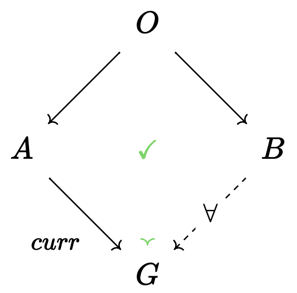
Weaken: switching to less specific agents
Weaken is specified by a morphism \(Hom_{C\mathsf{Set}}(A,B)\).
It converts \(B\)-agents to \(A\)-agents without changing the state of the world.
It acts upon an agent via precomposition.
Equivalent to a rewrite rule with \(A_{in} = L = I = R\)
Weaken: switching to less specific agents
Weaken is specified by a morphism \(Hom_{C\mathsf{Set}}(A,B)\).
It converts \(B\)-agents to \(A\)-agents without changing the state of the world.
It acts upon an agent via precomposition.
Equivalent to a rewrite rule with \(A_{in} = L = I = R\)
We can always weaken with the initial object:
Rewriting with initial agent is forgoing any explicit control of matches.
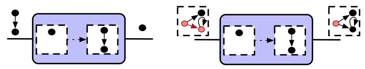
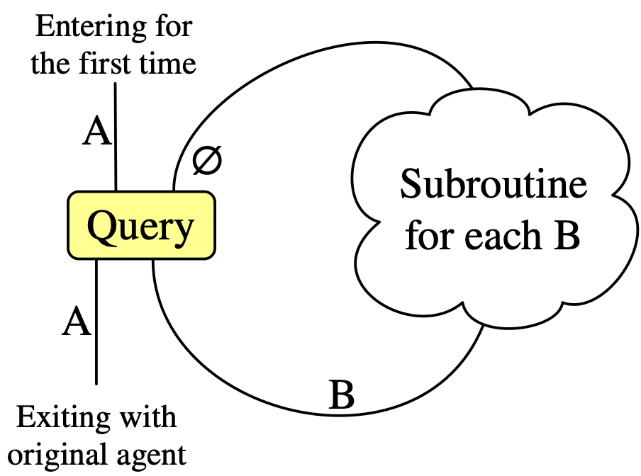
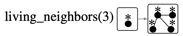
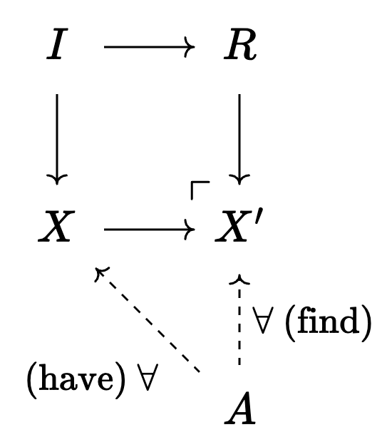
The Query primitive: more specific agents
Required data:
Example:
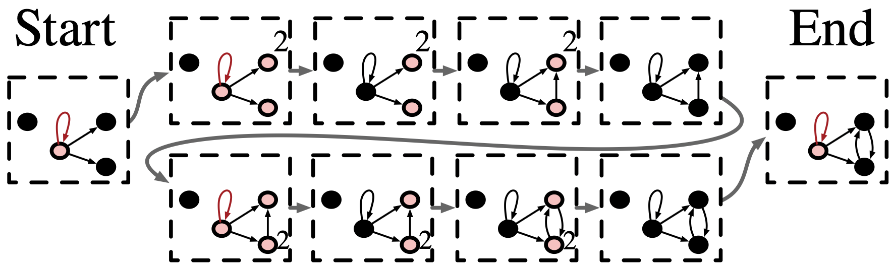
Fully connect all the outneighbor vertices of some distinguished loop
Summary of rewriting programs
Mealy machine primitives composed via directed wiring diagrams
Wires represent sets of morphisms \(A \rightarrow X\) for a fixed\(A\)
Changes are only performed by Rule
Shifting ‘agent’ focus performed by Query and Weaken
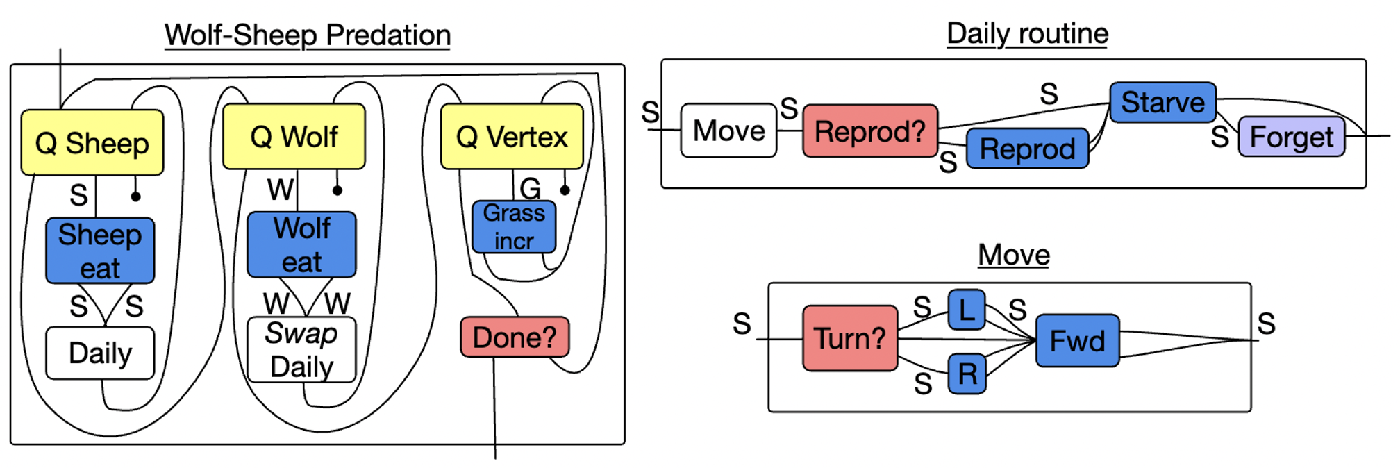
Implementing ABMs via agent-based programs
Why are these rewriting ‘programs’ rather than ‘models’?
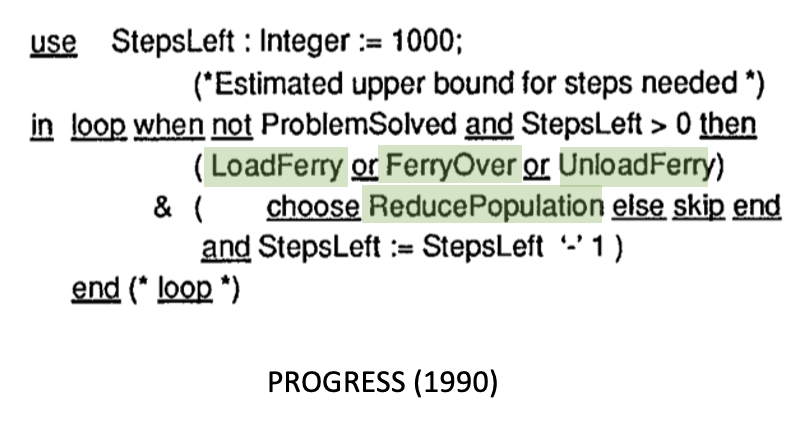
These feel less like programs compared to (equivalent) syntax like:
def simulate(X: Graph, steps: int) -> Graph:for step in steps:for match in homomorphisms(sheep, X):if length(homomorphisms(match, X)) >3: res = rewrite(rule5, match)if success(res): ...else: ...
Can be graphically depicted
Can be composed in parallel or in series
Can be operadically substituted
Can easily vary semantics
Nevertheless, this is not suited for agent-based modeling
Control flow fundamentally imperative rather than declarative.
To understand a diagram, you must run a simulation in your head.
No built-in notion of time
Always a linear sequence of events
No capability for concurrency
No capability for continuous time events
IV: Agent-based modeling1
These models are continuous time with discrete events and continuous dynamics.
To first order, an ABM is:
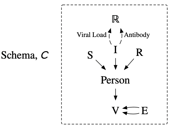
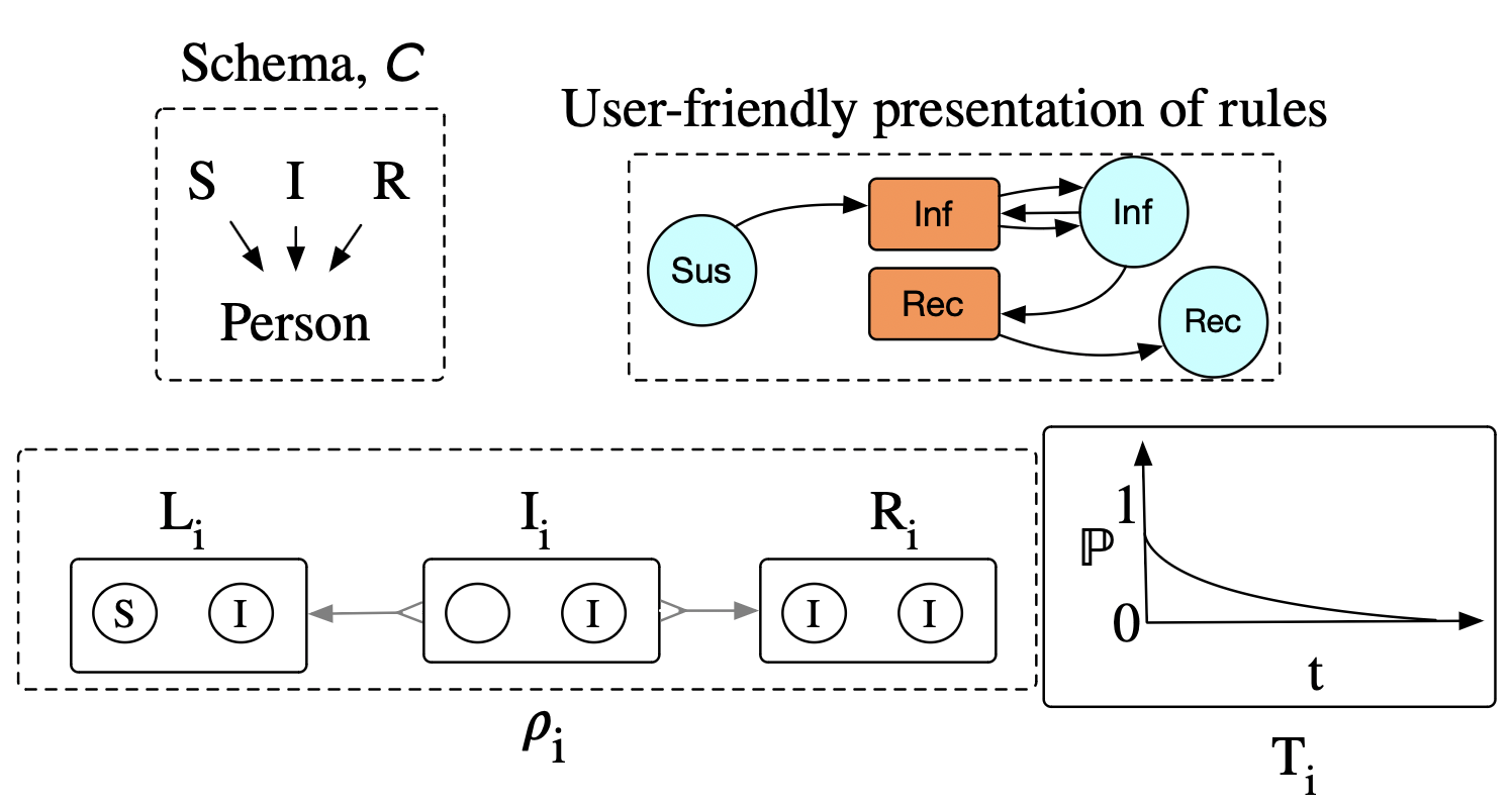
A schema: possible world states are ACSet instances
IV: Agent-based modeling1
These models are continuous time with discrete events and continuous dynamics.
To first order, an ABM is:
A schema: possible world states are ACSet instances
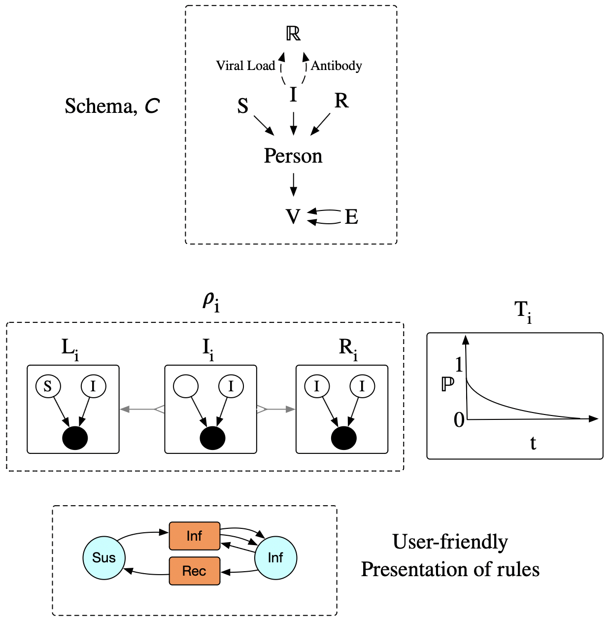
A collection of rewrite rules, \(\rho_i :: (L_i \leftarrowtail I_i \rightarrow R_i)\rightarrow \mathbf{ACSet}\)
An associated collection of ‘timers’ \(T_i :: \mathsf{P}([0,\infty])\).
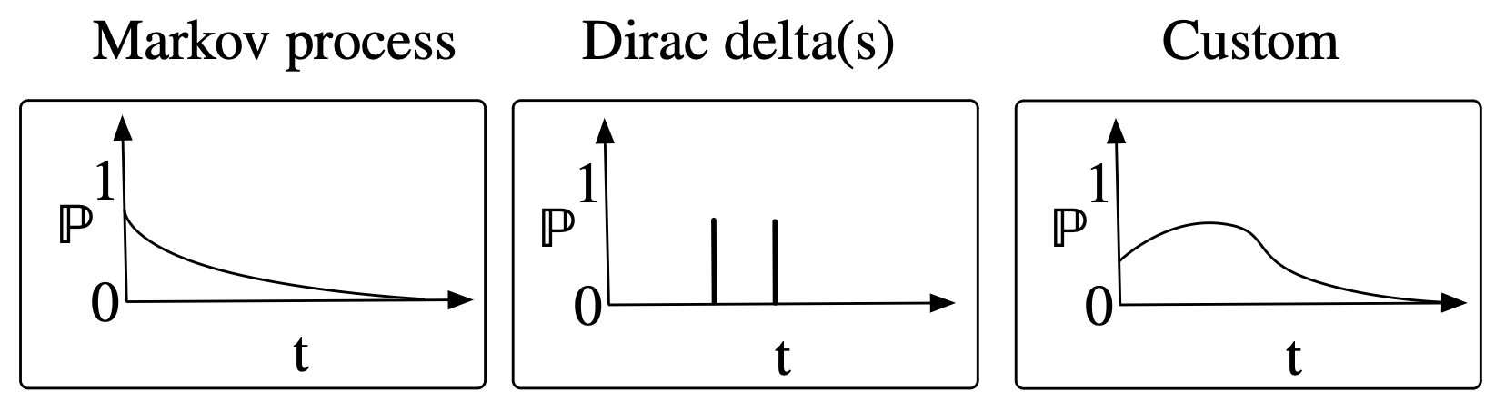
IV: Semi-Markovian ‘timers’
The probability measure captures a ‘residence time’:
how long it takes to happen, conditional on nothing else happening first to remove it from that state.
“staying in a state” = “match persists” over time
E.g.
Generalization: these are parameterized by the state of the world:
the probability of (\(S_i\), \(I_j\)) depends on the viral load of \(I_j\)
the probability of \(I_j\) recovering depends on the total # of doctors
IV: Agent-based modeling1
These models are continuous time with discrete events and continuous dynamics.
To first order, an ABM is:
A schema: possible world states are ACSet instances
A collection of rewrite rules, \(\rho_i :: (L_i \leftarrowtail I_i \rightarrow R_i)\rightarrow \mathbf{ACSet}\)
An associated collection of ‘timers’ \(T_i :: \mathsf{P}([0,\infty])\).
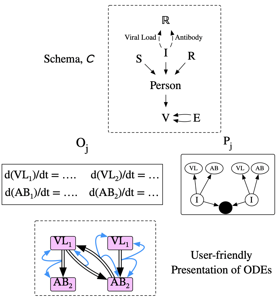
A collection of continuous dynamics, given by ODEs \(O_j\)
An associated collection of patterns, \(P_j :: \operatorname{Ob}(\mathbf{ACSet})\).
Partial functions from \(P_j\) variables to \(O_j\) variables.
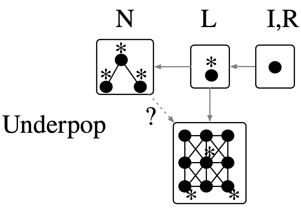
Example: Game of Life
@present SchLifeGraph <: SchSymmetricGraph begin Life::Ob; live::Hom(Life,V)end@acset_typeLifeState(SchLifeGraph); # defines LifeState# Helper functions / building blocks #-----------------------------------Cell =LifeState(1) # one vertex, nothing elseLiveCell =@acset LifeState begin V=1; Life=1; live=1endto_life =homomorphism(Cell, LiveCell);living_neighbors(n::Int; alive=true)::ACSetTransformation =...# Rules #------underpop =TickRule(:Underpop, to_life, id(Cell); ac=[NAC(living_neighbors(2))]);overpop =TickRule(:Overpop, to_life, id(Cell); ac=[PAC(living_neighbors(4))]);birth =TickRule(:Birth, id(Cell), to_life; ac=[PAC(living_neighbors(3; alive=false)),NAC(living_neighbors(4; alive=false)),NAC(to_life)]); # doesn't apply if aliveGoL =ABM([underpop, overpop, birth]) # model is just the rules
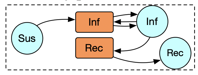
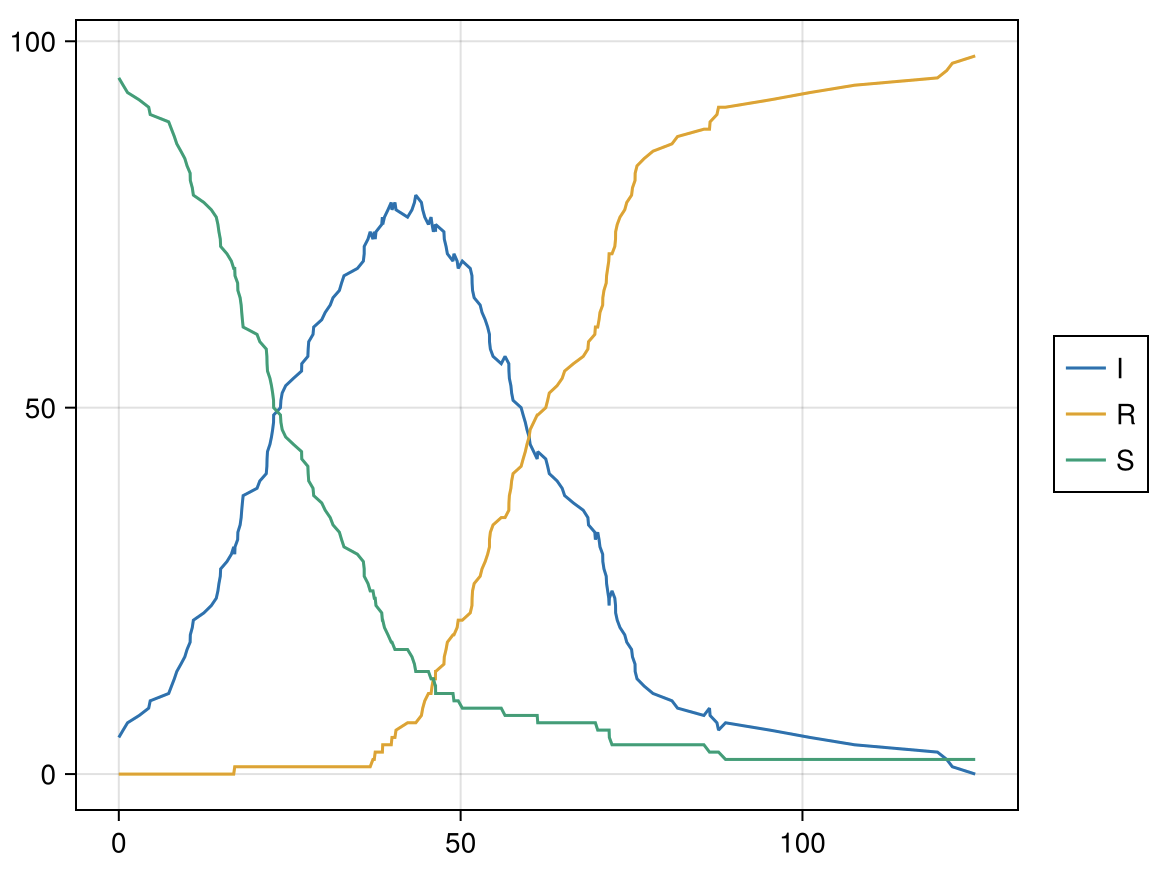
Example: Petri net token semantics
sir_pn =@acset LabelledPetriNet begin S=3; sname=[:S,:I,:R] T=2; tname=[:inf,:rec] I=3; is=[1,2,2]; it=[1,1,2]; O=3; os=[2,2,3]; ot=[1,1,2]end# Create ABM by associating stochastic timers with each Tabm =ABM(sir_pn, (inf=ContinuousHazard(1000), rec=ContinuousHazard(Weibull(30, 5)...)));# Initial stateinit =PetriNetCSet(sir_pn; S=95, I=5)# Run the modelres =run!(abm, init; maxtime=2000);
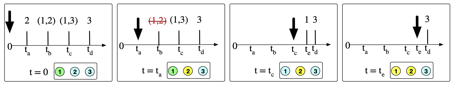
Performance: representable patterns
In certain circumstances, we don’t have to keep track of all the matches explicitly.
We have a simple exponential (memoryless) probability distribution
The pattern is a coproduct of representables (e.g. \(L = \bullet \oplus \bullet \rightarrow \bullet\))
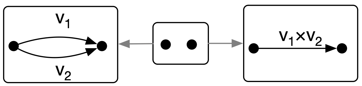
In this case, rather than draw a timer for every \((S, I)\) pair with probability \(e^{-kt}\), we draw just one timer with probability \(e^{-k*(|S|*|I|)t}\), then randomly pick a match at firing time.
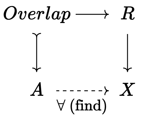
Performance: Incremental homomorphism search
For each overlap with \(R \setminus I\):
Synthesis of agent-based programs and models
One does not have to choose between ABP and ABM. In fact, we can use both:
Generalize the earlier definition of ABM: pairs of ABP+timer
Our previous formalism is a special case where all programs consist in just a single rule.
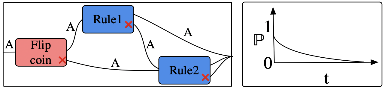
This lets us express things such as: after 5.0 s, something definitely happens, but which rule is applied depends on coin toss (or first one rule is tried, and a different is tried if that fails).
V: Conclusion
AlgebraicRewriting is expressive, powerful, easy to install, easy to use.
AlgebraicJulia is moving in a direction of factoring out our language-specific features, so that the same core can be instantiated in Python, Java, Rust, etc.
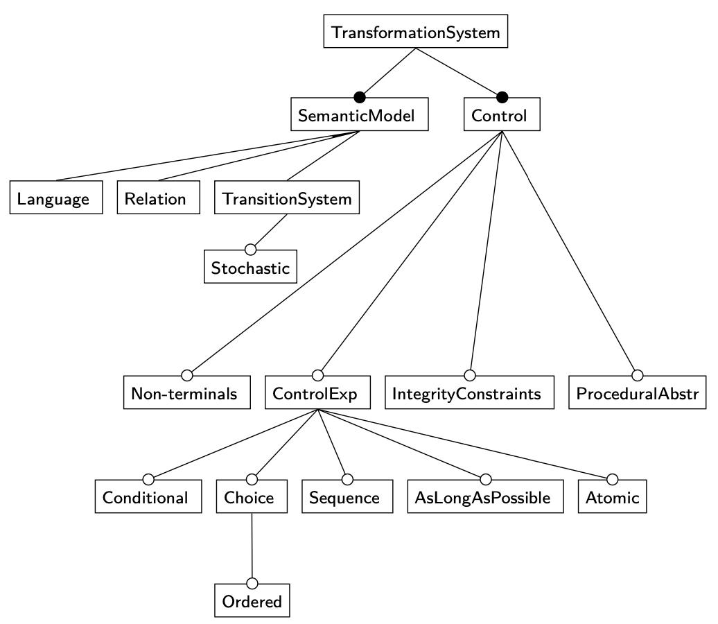
Graphical rewrite programs built from ControlFlow, Rewrite, Query, and Weaken
This syntax can be given a solid mathematical semantics.
Control flow + language for control over matches
Agent-based models can be constructed declaratively
A clear separation of schema, actions, and timing.
We could associate timers with entire programs, rather than individual rules.
This can be used for cellular automata, epidemiology, operations research
Manually, by specifying each component (e.g. V=[2,3], E=[1])
Via automated search + constraints, (e.g. monic=true)
CSet schemas (ACSet schemas)
DDS, Graph, Petri Net (ChemicalRxn)
Data migration:
Functor between schemas presents transformation process on instances
DDS to Graph, Graph to Petri Net
II. Catlab basics: category of directed multigraphs
Manually creating a graph
G =@acset Graph begin V=3; E=3; src=[1,1,2]; tgt=[1,2,2]end
Specifying via built-in constructors and coproducts
G =path_graph(Graph, 3) ⊕cycle_graph(Graph, 3)H =subobject_classifier(Graph) ⊕ob(terminal(Graph))
Manually specifying a graph homomorphism
h =ACSetTransformation(path_graph(Graph, 2), cycle_graph(Graph, 5); V=[2,3], E=[2])@testis_natural(h) # check naturality
Finding all homomorphisms \(X \rightarrow Y\) via automated search
hs =homomorphisms(X, Y; monic=[:E], # the edge component is injective, epic=[:V], # the vertex component is surjective, and initial=(V=Dict(2=>3),)) # X's V2 is mapped to Y's V3
II. Catlab basics: attributes
We are not limited to working with the category of directed multigraphs. Attributed C-Sets (ACSets) can have concrete attribute values in the ambient programming language.
@presentSchChemicalRxn(FreeSchema) begin (Atom, Bond, Molecule)::Ob# Functional relationships bond_atom::Hom(Bond, Atom) bond_pair::Hom(Bond, Bond) molecule::Hom(Atom, Molecule)# Equations bond_pair ⋅ bond_pair ==id(Bond)# Data types and attributes (N, ℝ)::AttrType atomic_number::Attr(Atom, N) stoichiometry::Attr(Molecule, ℝ)end
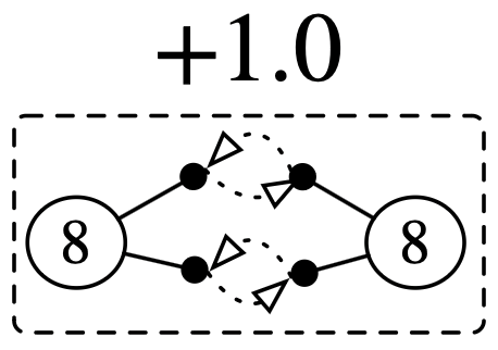
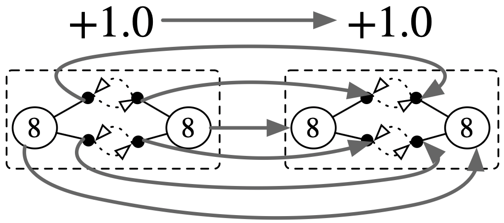
@acset_typeChemicalRxn(SchChemicalRxn){Int, Float64} O2 =@acset ChemicalRxn begin Atom=2; Bond=4; Molecule=1 bond_atom=[1,2,1,2]; bond_pair=[2,1,4,3] atomic_number=[8, 8]; molecule=[1,1] stoichiometry=[1.0]end# Get a symmetry of the molecule: swap the atomssigma =homomorphism(O2, O2; initial=(Atom=[2,1],))
II. Catlab basics: more schemas
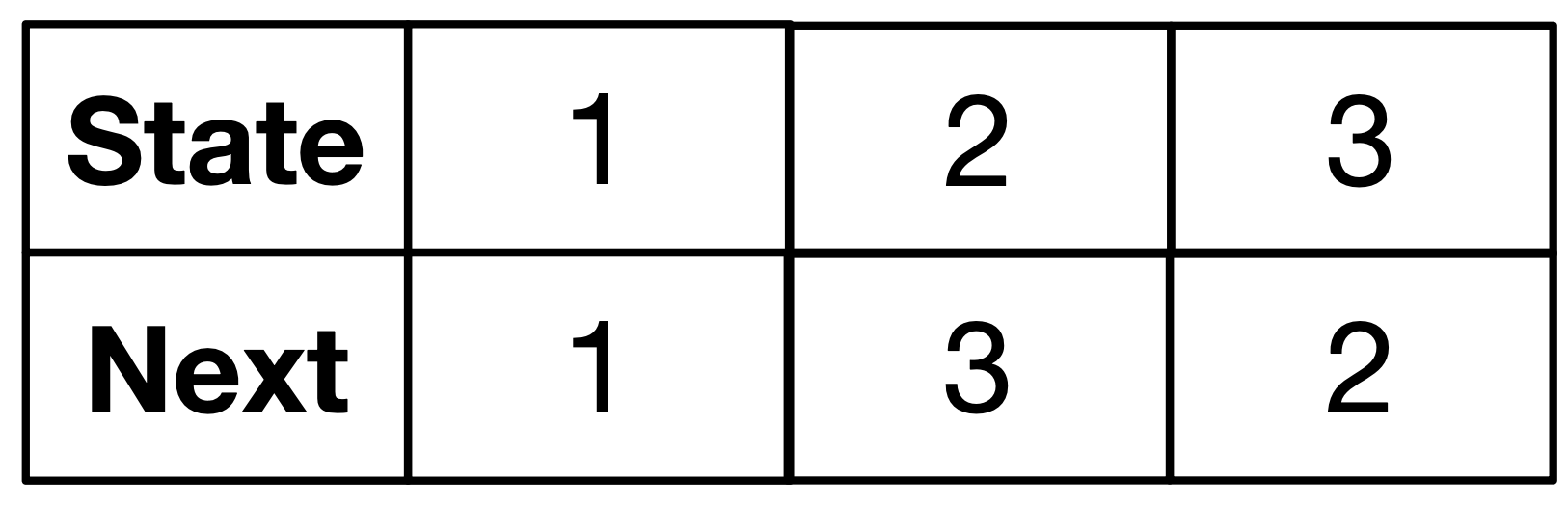
A discrete dynamical system as a set of states and a \(next\) function.
@presentSchDiscreteDynamicalSys(FreeSchema) begin State::Ob; next::Hom(State, State)end@acset_typeDDS(SchDiscreteDynamicalSys)
A petri net has a set of states, transitions, and input/output multirelations.
@presentSchPetriNet(FreeSchema) begin (S,T,I,O)::Ob; is::Hom(I, S); it::Hom(I,T); os::Hom(O, S); ot::Hom(O,T)end@acset_typePetriNet(SchPetriNet)
An example discrete dynamical system and example Petri net: