Representing sets and functions as data structures

B = set([False, True]) # builtin Python type

Colors = set(["red","green","blue"])

class Fun:
  def __init__(self, dom:set, codom:set, f:dict):
    self.dom = dom
    self.codom = codom
    self.f = f
  def __call__(self, v): 
    return self.f[v]

# builtin function
assert issubset(set(["a","b"]), set("c","b","a"))

def isomorphic(a:set, b:set): len(a) == len(b)

def image(f): 
  return set([f.f[a] for a in f.dom])

rg = Fun(Colors, B, {"red":True,"green":True,"blue":False})
gb = Fun(Colors, B, {"red":False,"green":True,"blue":True})
assert image(rg) == image(gb)

We’ve introduced some other data structures too:

class Graph:
  def __init__(self, src: Fun, tgt: Fun):
    assert src.dom == tgt.dom 
    assert self.codom == tgt.codom
    self.E = src.dom
    self.V = src.codom
    self.src = src
    self.tgt = tgt

class GraphHom:
  def __init__(self, vfun: Fun, efun: Fun):
    self.vfun = vfun 
    self.efun = efun

class Petri:
  def __init__(self, i_s: Fun, i_t: Fun, o_s: Fun, o_t: Fun):
    assert i_s.dom == i_t.dom and i_s.codom == o_s.codom
    assert o_s.dom == o_t.dom and i_t.codom == o_t.codom
    self.S, self.T = i_s.codom, i_t.codom
    self.I, self.O = i_s.dom, o_s.dom
    self.i_s, self.i_t = i_s, i_t
    self.o_s, self.o_t = o_s, o_t

class PetriHom:
  def __init__(self, sfun, tfun, ifun, ofun):
    self.sfun = sfun
    ...

set automatically handles deduplication.

Set theory

The cardinality of a set \(|A|\) measures the number of elements in the set.

\(|\{red, green, blue\}|=3\)

\(|\B|=2\)

\(|\{\}| = 0\)

\(|\{\bullet \}| = 1\)

\(|\N| = \infty\)

. . .

Set theory: definitions

The identity function for a set \(X\) sends each \(x \in X\) to itself.

The composition of functions \(f: A\rightarrow B\) and \(g: B \rightarrow C\) is a function \(f \then g: A \rightarrow C\) which sends each \(a \in A\) to \(g(f(a))\).

Set theory: on the computer

id(X::Set) = Fun(X, X, Dict(x=>x for x in X))
compose(f::Fun, g::Fun) =
  Fun(f.dom, g.codom, Dict([a=>g.fun[f.fun[a]] for a in f.dom]))

def id(X): Fun(X, X, {x:x for x in X})
def compose(f, g): return Fun(f.dom, g.codom, 
  {a : g.fun[f.fun[a]] for a in f.dom})

Set theory: definitions

An injective function does not send distinct elements in \(A\) to the same element of \(B\).

\(\forall a,a' \in A, a\ne a' \implies f(a) \ne f(a')\)

A surjective function has for each element in \(B\) some element of \(A\) mapping to it.

\(\forall b \in B, \exists a \in A, f(a)=b\)

\(im(f) = B\)

A bijective function is one which is both injective and surjective.

…

Set theory: theorems

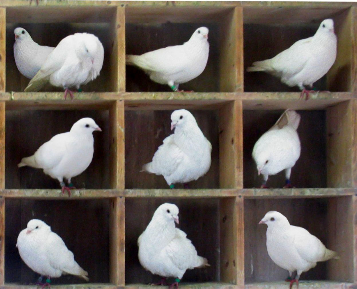
For any \(f: A\rightarrow B\), if \(|A| > |B|\) then \(f\) is not injective.

Any lossless compression algorithm which makes some inputs smaller will also make some other inputs larger.

…

Set theoryII: examples

injective(f::Fun) = length(image(f)) == length(f.dom)
surjective(f::Fun) = length(image(f)) == length(f.codom)
bijective(f::Fun) = injective(f) && bijective(f)

def injective(f): 
  return len(image(f)) == len(f.dom)
def surjective(f): 
  return len(image(f)) == len(f.codom)
def bijective(f): 
  return injective(f) and bijective(f)

Julia isn’t that different from Python. Should be straightforward to pick up.

Set theoryV: definitions

The intersection of sets.

\(X \cap Y := \{elem\ |\ elem \in X \land elem \in Y\}\)

The union of sets.

\(X \cup Y := \{elem\ |\ elem \in X \lor elem \in Y\}\)

…

Set theoryV: definitions

The product (cartesian product) of sets

\(X \times Y := \{(x,y)\ |\ x \in X \lor y \in Y\}\)

The coproduct (disjoint union) of sets

\(X + Y := \{(x,y)\ |\ x \in X \lor y \in Y\}\)

The exponential of sets

\(Y^X := \{f\ |\ f:X \rightarrow Y\) is a function \(\}\)

…

Set theoryV: theorems

These operations are symmetric and associative:

\(A \cap B = B \cap A\)

\(A \cup B = B \cup A\)

\(A \times B \cong B \times A\)

\(A + B \cong B + A\)

\((A \cap B) \cap C = A \cap (B\cap C)\)

\((A \cup B) \cup C = A \cup (B\cup C)\)

\((A \times B) \times C \cong A \times (B \times C)\)

\((A + B) + C \cong A + (B + C)\)

These operations are natural with respect to cardinality:

\(|A + B| = |A| + |B|\)

\(|A \times B| = |A| \times |B|\)

\(|B^A| = |B|^{|A|}\)

This means we can interpret arithmatic equalities as isomorphisms of sets!

\(Z^{X+Y} \cong Z^X \times X^Y\)

Category theory: definitions

A small category \(C\) consists of

• a set \(C_0\) of objects
• for every \(x,y \in C_0\), a set \(\mathrm{Hom}_C(x,y)\) of morphisms from \(x\) to \(y\)
• for every \(x,y,z \in C_0\), a composition function \(\then \colon \mathrm{Hom}_C(x,y) \times \mathrm{Hom}_(y,z) \to \mathrm{Hom}(x,z)\)
• for every \(x \in C_0\), an identity morphism \(1_x \in \mathrm{Hom}_C(x,x)\)

such that

• for all \(x,y,z,w \in C_0\), \(f \in \mathrm{Hom}_C(x,y)\), \(g \in \mathrm{Hom}_C(y,z)\), \(h \in \mathrm{Hom}_C(z,w)\), \[ f \then (g \then h) = (f \then g) \then h \]
• for all \(x,y \in C_0\), \(f \in \mathrm{Hom}_C(x,y)\), \[ 1_x \then f = f = f \then 1_y \]

These two laws are called the associativity law and unitality law respectively.

Category theory: examples

With a little practice, it’s easy to look at something and understand it as a category (as it is to look at something and see it as a set of things, connected via functions).

Category theorys useful because common, useful abstractions in different settings end up being revealed to have the same structure. We can use that when programming to have a single implementation.

Some examples of categories we have seen so far:

Category	Ob	Hom	Id	Comp
Set	sets	functions \(f: A\rightarrow B\)	identity function	function composition
Grph	graphs	graph maps	identity map	map composition
Petri	Petri nets	Petri maps	identity map	map composition
Sub(X)	subsets of \(X\)	inclusions	identity function	function composition
Mat	\(\N\)	\(n \times m\) matrices	e.g. \(\begin{pmatrix}1 & 0 \\ 0 & 1 \end{pmatrix}\)	matrix multiplication
Nat	\(\N\)	\(n \leq m\) relation	\(\leq\) reflexivity	\(\leq\) transitivity

Thinking categorically

In Set, the empty set is distinctive (initial) because it has exactly one function into every other set. The singleton set is terminal because it has exactly one function into it from every other set.

We can understand these notions of initial and terminal in other categories:

Category	Ob	Hom	Initial	Terminal
Set	sets	functions \(f: A\rightarrow B\)	\(\{\}\)	\(\{\bullet\}\)
Grph	graphs	graph maps	?	?
Petri	Petri nets	Petri maps	?	?
Sub(X)	subsets of \(X\)	inclusions	?	?
Mat	\(\N\)	\(n \times m\) matrices	?	?
Nat	\(\N\)	\(n \leq m\) relation	?	?

Category theory shows how operations like \(\subseteq\), \(\cap\), \(\cup\), \(+\), \(\times\), \(\cong\), exponential, pushout, pullback … all have characterizations like initial and terminal which make sense in any category.

Petri nets and chemical reaction networks: multiplication

Previously, we had a model sys representing a metal solution oxidizing in a beaker in an atmosphere of \(O_2\) and \(N_2\). We’ve now realized there are two beakers with different solutions, and we want to duplicate that part of the reaction network (without duplicating the atmosphere and its reactions).

# Representation of duplication possibilities
base = LabelledPetriNet([:Dup,:NoDup], 
  :dup => (:Dup,:NoDup)=>(:Dup,:NoDup), 
  :nodup => (:Dup,:NoDup)=>(:Dup,:NoDup))
to_graphviz(base)

Petri nets and chemical reaction networks: pullback

# Representation of duplication
dup = LabelledPetriNet([:Dup1,:Dup2,:NoDup], 
    :dup1 => (:Dup1,:NoDup)=>(:Dup1,:NoDup),  
    :dup2 => (:Dup2,:NoDup)=>(:Dup2,:NoDup), 
    :nodup => (:Dup1,:Dup2,:NoDup)=>(:Dup1,:Dup2,:NoDup))
to_graphviz(dup)

AB,AS,AD= abstract_attributes.([base,sys,dup])
abs_base,abs_sys,abs_dup = dom.([AB,AS,AD])
sys_base = homomorphism(PetriNet(abs_sys),PetriNet(abs_base); initial=(S=[2,2,2,1,1], T=[1,2]))
dup_base = homomorphism(PetriNet(abs_dup),PetriNet(abs_base); initial=(S=[1,1,2], T=[1,1,2]))
pullback(sys_base,dup_base) |> apex |> to_graphviz

ODEs

Up until this point we manipulated Petri Nets as implicit presentations of ordinary differential equations. Now we consider ODEs in general and how we wish to compose them.

Logic Notation

Propositional logic:

• \(p \land q\) - “The proposition \(p\) and \(q\)”
• \(p \lor q\) - “The proposition \(p\) or \(q\)”

• \(\neg p\) - “The proposition not-\(p\)”
• \(p \implies q\) - “The proposition \(p\) implies \(q\)”

• \(E\) = “My favorite # is even”
• \(O\) = “My favorite # is odd”
• \(D\) = “My favorite # is divisible by 4.”

\(D \implies E\)

\(E \lor O\)

\(E \iff \neg O\)

. . .

Predicate logic:

• \(\forall x \in X: \phi(x)\) — “For all \(x\)’s in \(X\), it is the case that \(\phi\) of \(x\) is true”
• \(\exists x \in X: \phi(x)\) — “There exists an \(x\) in \(X\), such that \(\phi\) of \(x\) is true”

• \(E(x)\) = “x is even”
• \(O(x)\) = “x is odd”
• \(D(x)\) = “x is divisible by 4.”

\(\forall x \in \N: O(x) \lor E(x)\)

\(\neg \exists x \in \N, D(x) \land O(x)\)

\(\forall x,y \in \N: E(x)\land O(y)\implies O(x+y)\)

Note that or is inclusive.

Implicitly we are quantifying over natural numbers in the bottom.

Comprehension check

Let \(\phi(x) := x^2-2 = 0\) and \(\psi(x) := x \in \Q\)

Which statement is true? (tip: translate \(\phi\) and \(\psi\) to plain English first!)

A.) \(\exists n \in \R: \phi(n) \land \psi(n)\)

B.) \(\forall n \in \R: \phi(n) \lor \psi(n)\)

C.) \(\forall n \in \R: \phi(n) \implies \neg \psi(n)\)

D.) \(\exists n,m \in \R: \phi(n) \land \psi(m) \land \psi(n)\)

. . .

Two kinds of scientific modeling problems

1. How do we represent the math on the computer?
2. How do we efficiently compute solutions?

Category theory is a branch of math which is suited for addressing the first problem. It is the mathematics of structure, or of composition.

It guides us in telling us exactly what we have to implement in order to write code to do the sorts of compositions in the motivating examples (much like the theory of ODEs taught in this course instructs us how to analytically and numerically solve ODEs).

Another advantage of thinking category theoretically: it helps us write general / generalizable code. For example, it tells us an abstract structure of ‘product’, which we can instantiate in many settings.

• \(A \& B\) for boolean logic
• Intersection of sets, \(A \cap B\)
• Multiplication of numbers, \(A \times B\)
• Multiply spaces, e.g. circle \(\times\) line = cylinder

• Greatest common divisor \(gcd(A,B)\)
• Pair type \((A,B)\) in a programming language
• Greatest lower bound in a hierarchy
• Construct block matrix \(\begin{pmatrix}A & 0 \\ 0 & B \end{pmatrix}\)

Here are examples of ways to structure various mathematical models. On the left we have “directed wiring diagram”, on the right we have an “undirected wiring diagram”.

These are examples of “graphical syntax”. Understanding these as formal mathematical objects (which category theory allows us to do), we can very cleanly write the code once required to make them work in a variety of settings.

We also have a notion of “the structure of a product” which can be instantiated in many different settings to recover familiar operations.

Two kinds of scientific modeling problems

1. How do we represent the math on the computer?
2. How do we efficiently compute solutions?

Scientific programming traditionally prioritizes being able to answer the second question. This course focuses on mathematics of analysis, calculus, and linear algebra, which are obviously useful for this. Yet abstract algebra (e.g.  group theory, ring theory) can be useful for this:

. . .

Gröbner basis, solving kinetics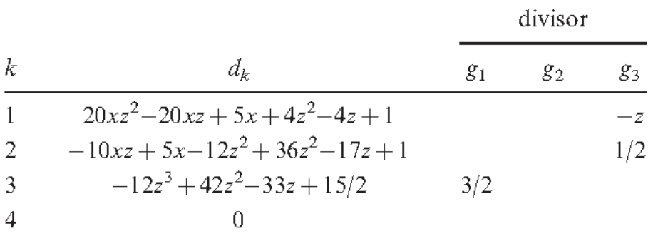

Point groups, raman spectroscopy

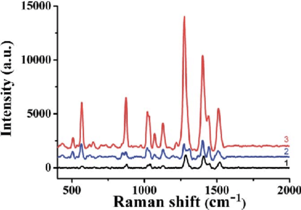
When solving problems on a computer, we have to worry about these two questions.

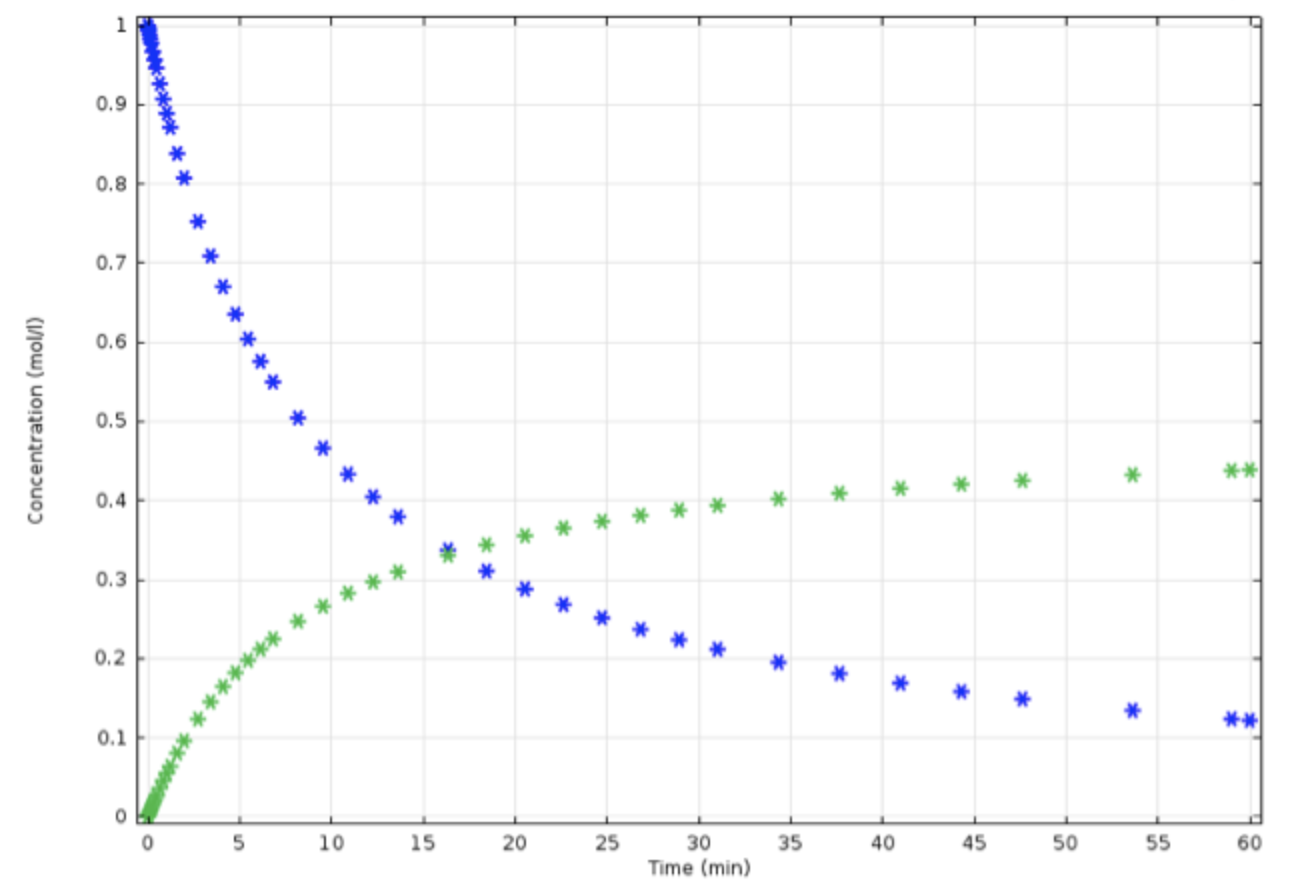
• Gröbner basis / Buchberger algorithm computes analytic solutions to chemical reaction networks.

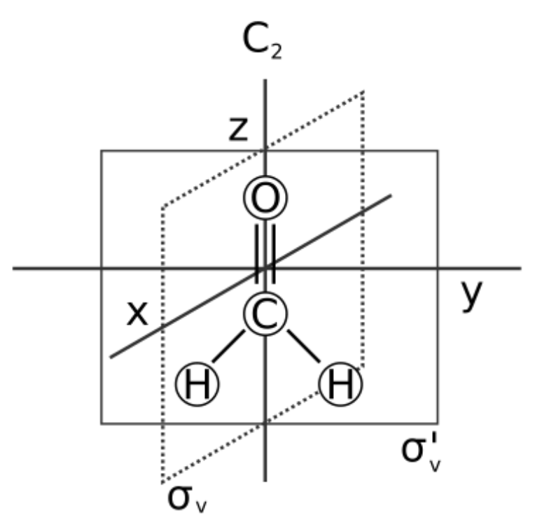
• Point groups describe molecular symmetries, providing qualitative predictions about the possible vibrations (and therefore spectroscopy results)

Motivating example: another system composition

def more_reactions(time):
  V1, V2, V3, V4 = 20.0, 30.0, 20.0, 30.0 # L
  in_concs = [996, 0.4, 0.05, 0.05] # g/L

  def yprime(t, concs):
    H2O2_1, H2O_1, H_1, ..., H2O2_2, ... = concs
    # NEW MATH TO BE WORKED OUT  
  
  solve_ivp(yprime, [0, time], [.1,.4,.3,.5])

@relation 
def glue_three_crns():
  crn1(overlap1, overlap2)
  crn2(overlap1, overlap2)
  crn3(overlap2)

olap1_1 = ...
olap1_2 = ...

def more_reactions(): # much nicer
  return compose(glue_three_crns, 
                 [[olap1_1, olap1_2], 
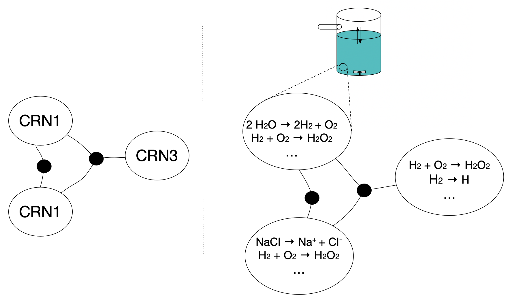
                  [olap2_1, olap2_2, olap2_3]])

Another way Aditi could be cruel is to at the last second change the chemical reaction network. The network might be expressed as three different networks which are glued along some common boundaries, represented as black dots. Think of three different partial descriptions of the whole which need to be assembled together.

For example, you might have the gas phase reactions together, the the liquid phase reactions, the reactions/mass transfer at the interface, each designed by different teams. But the teams then need to come together, combining their work (which might have lots of conflicting naming and redundancy).

Comprehension check

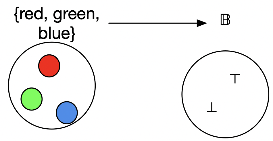
How many functions are there from \(\{red, green, blue\}\) to \(\B\)?

A.) 3

B.) 6

C.) 8

D.) 9

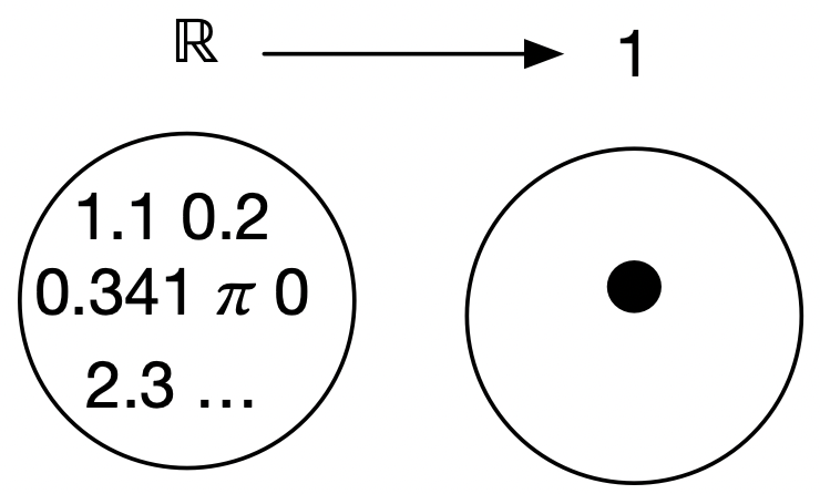
How many functions are there from \(\R\) to \(1\)?

A.) 0

B.) 1

C.) \(|\N|\)

D.) \(|\R|\)

Bonus question, what are some sets \(A,B\) such that there are || functions \(A \rightarrow B\)?

Set theory: definitions

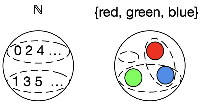
A subset of a set.

\(X \subseteq Y := \forall x \in X, x \in Y\)

• \(Evens \subseteq \N\), \(Odds \subseteq \N\)
• \(\{\} \subseteq \{red,green,blue\}\)
• \(\{red, blue\} \subseteq \{red,green,blue\}\)
• \(\{green, blue\} \subseteq \{red,green,blue\}\)

The image of a function \(f: A \rightarrow B\) is the subset of \(B\) mapped to by \(f\).

\(im(f) := \{f(a)\ |\ a \in A\}\)

• \(im(double: \N\rightarrow\N) = Evens\)
• \(im(\#ofLettersIsOdd: \{red,green,blue\}\rightarrow \B) = \B\)
• \(im(x\mapsto x^2: \R\rightarrow\R) = \R^{\geq 0}\)