Building computational models via structural mathematics

Kris Brown

(press s for speaker notes)

3/6/24

Outline

I. Future of software engineering

II. Mini examples of the future paradigm

III. Intuition for how structural mathematics works

Note: it’s not feasible to cover category theory at a technical level in such a short talk, rather I want to show what you can do with it. So I’ll be avoiding jargon whenever possible, including the phrase “category theory” itself! Rather, we should just think of category theory as ‘the mathematics of structure’: something that makes precise our intuitions about structure in a way that allows us to actually compute things.

Stages of development for software engineering

1. We solve problems one at a time, as they come.

This starts feeling repetitive.

2. Abstractions act as a solution to an entire class of problems.

This feels repetitive insofar as we feel the problem classes are related.

Common abstractions are things like functions / datatypes / scripts in our language.

3. We migrate abstractions to allow them to address changes in problem specification.

Future paradigm: mathematically-principled + automatic abstraction reuse

Understand structure of the abstraction + implementation + the relationship between them.

This slide summarizes everything I want to talk about today. (Stage 1)

(…) (Stage 2)

(…) (Stage 3)

There will be lots of examples illustrating how we can move from Stage 2 to 3 when we use abstractions that we understand well. I’ll try to clearly show what’s going on for toy examples and then (at the end) Evan will showcase some real, practical examples at a high level.

Three examples of abstractions

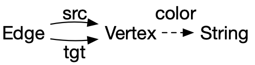
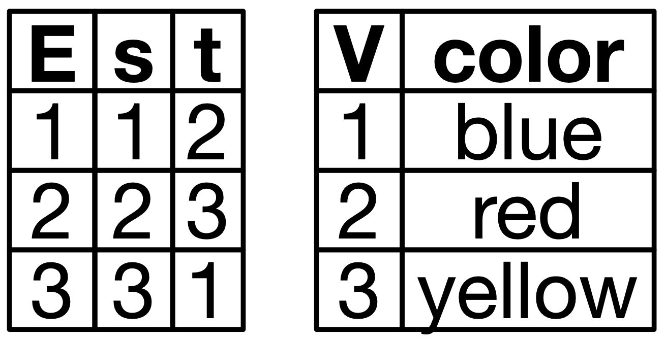
In this section of the talk: I’ll make reference to three specific types of abstractions which I’ll introduce one at a time. These are databases (here I’m just showing a particular toy database schema), Petri nets (also called bipartite graphs), and wiring diagrams

Abstraction: databases (SQL)

CREATE SCHEMA COLORGRAPH;
CREATE TABLE VERT (ID PRIMARY KEY, COLOR VARCHAR);
CREATE TABLE EDGE (ID PRIMARY KEY, 
                   FOREIGN KEY TGT REFERENCES VERT(ID),
                   FOREIGN KEY SRC REFERENCES VERT(ID));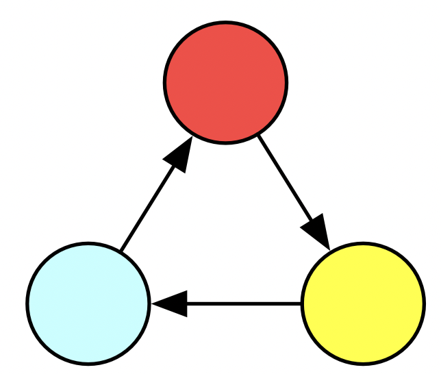

INSERT INTO VERT VALUES ('B')
INSERT INTO VERT VALUES ('R')
INSERT INTO VERT VALUES ('Y')
INSERT INTO EDGE VALUES (1,2)
INSERT INTO EDGE VALUES (2,3)
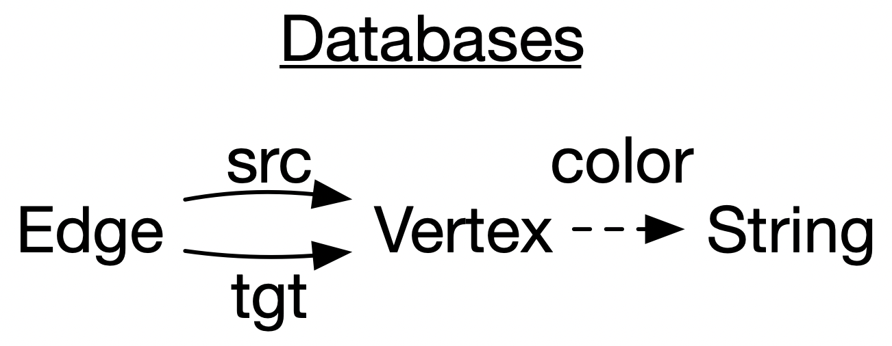
INSERT INTO EDGE VALUES (3,1)

Here is an example specific database schema. Schemas are abstractions which codify various logical constraints, such as “every edge has a source and target vertex” and “every vertex has a color”.

Below are two representations of a particular instance of this database. To the right are some SQL statements which would create such a triangle.

Abstraction: databases (Julia)

struct ColorGraph
  edges::Set{Pair{Int, Int}}
  vertices::Set{Int}
  colors::Dict{Int, String}
end

@present SchColorGraph begin
  (V, E) :: Ob; (src, tgt) :: Hom(E, V)
  Color :: AttrType; color :: Attr(V, Color)
end
@acset_type ColorGraph(SchColorGraph){String}

function triangle!(graph=ColorGraph())
  a, b, c = [add_vertex!(graph, color)  
             for color in "BRY"]
  [add_edge!(graph, s, t) for 
    (s, t) in [[a,b],[b,c],[c,a]]]
  return graph
end

New problem expressed in terms of old problem.

In addition to the SQL way of framing this, we could also do this with a class or struct, though admittedly that would not capture the foreign key requirements. On the right, I show how we declare this data structure in AlgebraicJulia, which is declaring the database schema. (…)

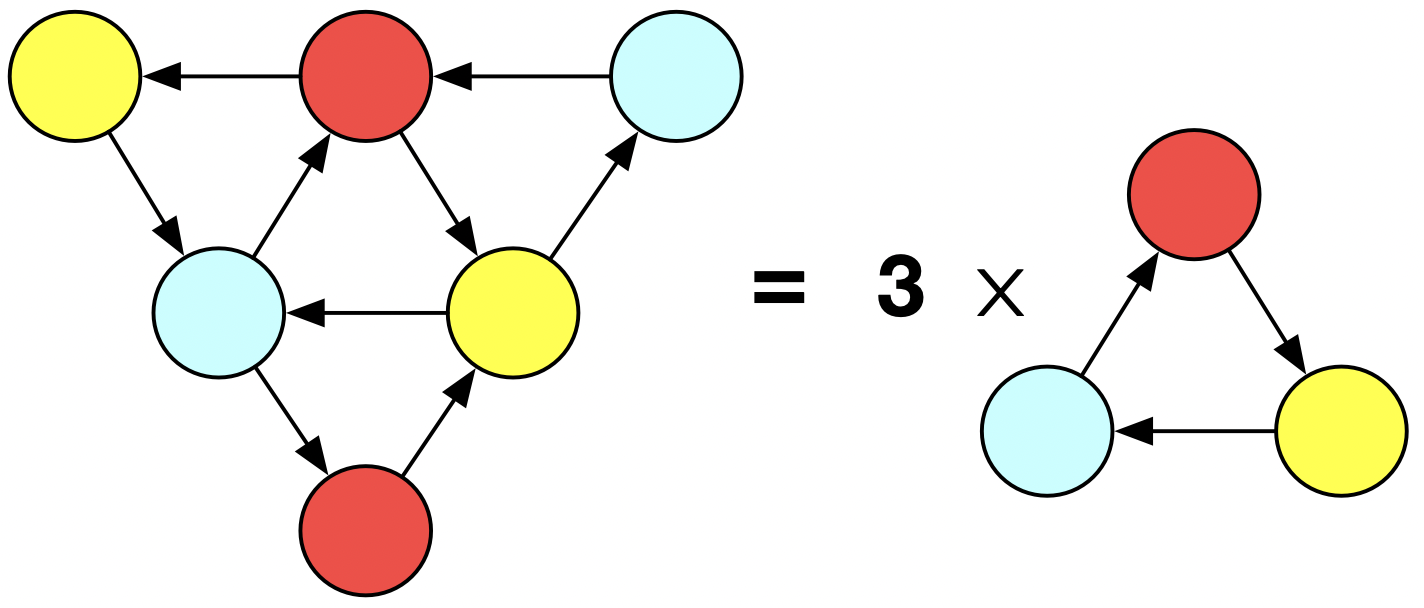
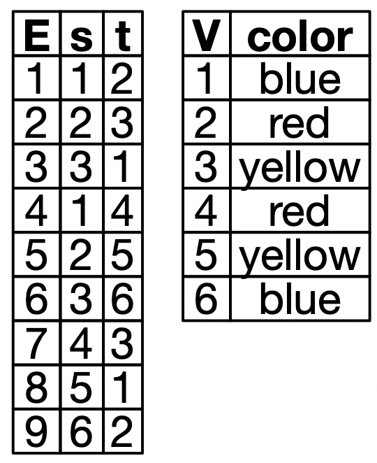
For our first concrete example of abstraction reuse: consider this big triangle. We could always just code this up again from scratch, but what if we recognize that the big triangle is just three different triangles that have been glued together? It’s a mark of a good abstraction for our triangle function that it permits us to do this.

Gluing: side-by-side comparison

"""Modify to allow it to overlap existing vertex IDs"""
function triangle!(graph, v1=nothing, v2=nothing, v3=nothing)
  vs = map([v1=>"B", v2=>"R", v3=>"Y"]) do (v, color)
    isnothing(v) ? add_vertex!(graph, color) : v
  end
  [add_edge!(graph, vs[i]...) for i in [1:2,2:3,[3,1]]]
  vs
end

"""Now expressible as an abstraction of `triangle!`"""
function big_tri!(graph)
  blue, red, _ = triangle!(graph)
  _, _, yellow = triangle!(graph, blue)
  triangle!(graph, nothing, red, yellow)
end

function replace!(graph, fk::Symbol, 
                  find::Int, repl::Int)
end # TODO

function big_tri!(graph)
  triangle!(graph)
  triangle!(graph)
  triangle!(graph)
  for fk in [:src, :tgt]
    replace!(graph, fk, 5, 2)
    replace!(graph, fk, 7, 1)
    replace!(graph, fk, 9, 5)
  end
  [rem_vertex!(graph, v) for v in [5,7,9]]
end

Here are two different ways we could leverage our triangle! function to make a big colored triangle, thought of as three colored triangles which a related by a kind of gluing relationship.

The first one requires us to modify triangle!. No longer does it just add a triangle to some preexisting database instance, but it allows one to pass in parameters so that the triangle has the option of reusing existing vertices. Not only did we have to substantial refactor of the function, it was also convenient to change the behavior of the old function a bit (by having it return vertices rather than the graph itself), so there may be other places in our codebase where we have to fix broken code.

The second one doesn’t require us to modify the function: it just creates three disjoint triangles, and then ‘manually’ modifies the result to manipulate the foriegn keys and finally delete the isolated vertices. Although we did not need to modify the function, we certainly needed a deep understanding of its implementation in order to do this, plus this code is very clunky and not at all re-usable for other problems (whereas the first solution has potential to be used for other compositions of triangles).

Gluing: side-by-side comparison

"""Modify to allow it to overlap existing vertex IDs"""
function triangle!(graph, v1=nothing, v2=nothing, v3=nothing)
  vs = map([v1=>"B", v2=>"R", v3=>"Y"]) do (v, color)
    isnothing(v) ? add_vertex!(graph, color) : v
  end
  [add_edge!(graph, vs[i]...) for i in [1:2,2:3,[3,1]]]
  vs
end

"""Now expressible as an abstraction of `triangle!`"""
function big_tri!(graph)
  blue, red, _ = triangle!(graph)
  _, _, yellow = triangle!(graph, blue)
  triangle!(graph, nothing, red, yellow)
end

function replace!(graph, fk::Symbol, 
                  find::Int, repl::Int)
end # TODO

function big_tri!(graph)
  triangle!(graph)
  triangle!(graph)
  triangle!(graph)
  for fk in [:src, :tgt]
    replace!(graph, fk, 5, 2)
    replace!(graph, fk, 7, 1)
    replace!(graph, fk, 9, 5)
  end
  [rem_vertex!(graph, v) for v in [5,7,9]]
end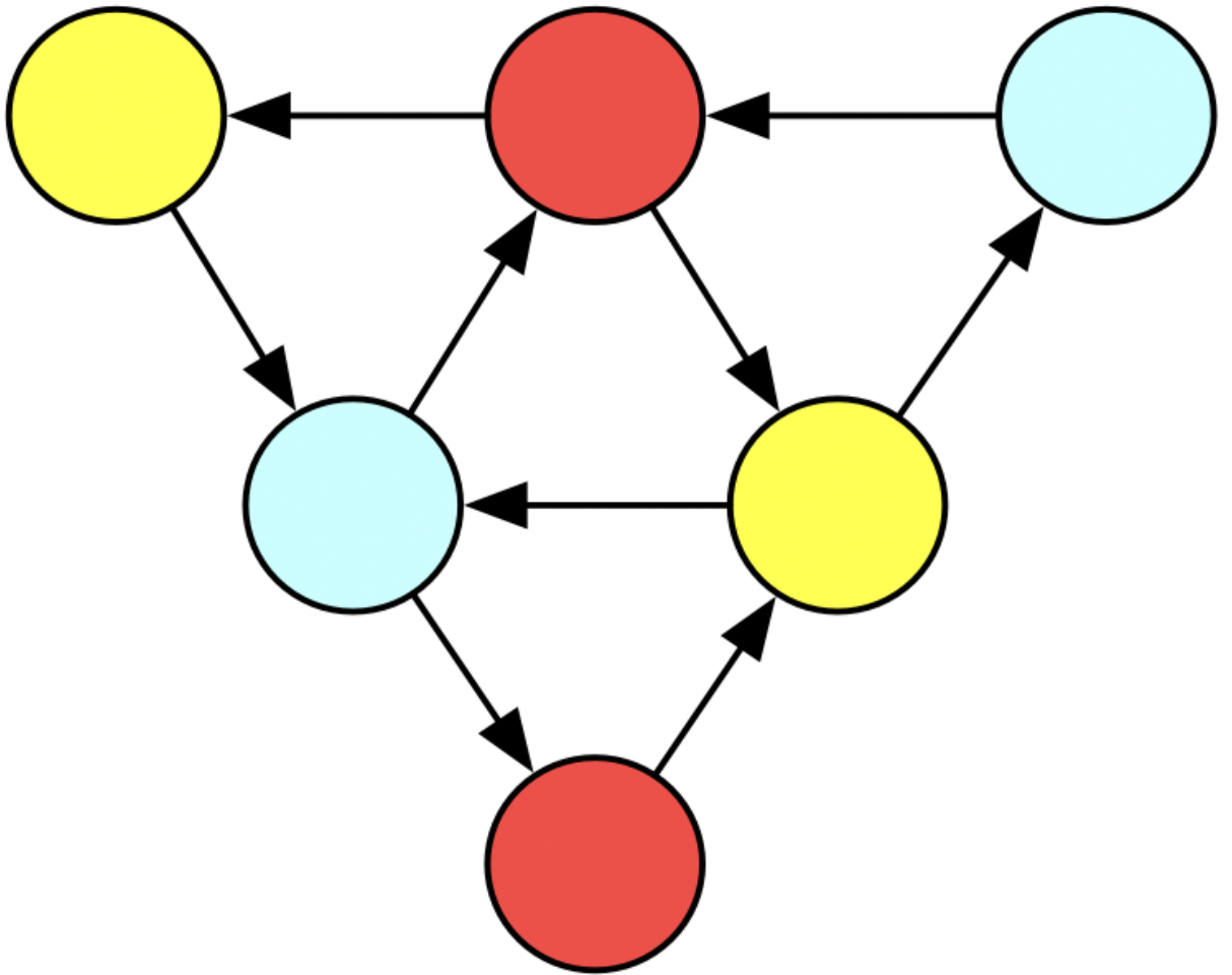

AlgebraicJulia

# Building blocks
T1,T2,T3 = [triangle!() for _ in 1:3]
b,r,y = [add_vertex!(ColorGraph(), c) for c in "BRY"]

# Relation of building blocks to each other
pattern = @relation (;) where (t1, t2, t3) begin
  b(t1, t2); r(t2, t3); y(t3, t1)
end

# Composition
big_tri = glue(pattern; T1, T2, T3, b, r, y)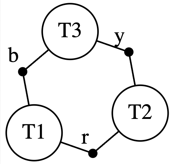

On the bottom here I have some code built on top of AlgebraicJulia. We construct the big triangle in three steps. We declare the building blocks, we declare how those building blocks are related to each other, and then we compose the building blocks according to the relation. On the right I show what we call an undirected wiring diagram - this is what is created in line 6. We are going to stick triangles into T1, T2, T3, and we will stick an isolated vertex of the appropriate color in b, r, and y. The lines in the diagram say that b must be related to T1 and T3 in some way. It turns out there is only one way this can be done, by mapping the blue vertex to the blue vertex of the T1 (and of T3). So there is no further information needed to disambiguate what composing these building blocks means.

Gluing: side-by-side comparison

"""Modify to allow it to overlap existing vertex IDs"""
function triangle!(graph, v1=nothing, v2=nothing, v3=nothing)
  vs = map([v1=>"B", v2=>"R", v3=>"Y"]) do (v, color)
    isnothing(v) ? add_vertex!(graph, color) : v
  end
  [add_edge!(graph, vs[i]...) for i in [1:2,2:3,[3,1]]]
  vs
end

"""Now expressible as an abstraction of `triangle!`"""
function big_tri!(graph)
  blue, red, _ = triangle!(graph)
  _, _, yellow = triangle!(graph, blue)
  triangle!(graph, nothing, red, yellow)
end

function replace!(graph, fk::Symbol, 
                  find::Int, repl::Int)
end # TODO

function big_tri!(graph)
  triangle!(graph)
  triangle!(graph)
  triangle!(graph)
  for fk in [:src, :tgt]
    replace!(graph, fk, 5, 2)
    replace!(graph, fk, 7, 1)
    replace!(graph, fk, 9, 5)
  end
  [rem_vertex!(graph, v) for v in [5,7,9]]
end

AlgebraicJulia

# Building blocks
T1,T2,T3 = [triangle!() for _ in 1:3]
b,r,y = [add_vertex!(ColorGraph(), c) for c in "BRY"]

# Relation of building blocks to each other
pattern = @relation (;) where (t1, t2, t3) begin
  b(t1, t2); r(t2, t3); y(t3, t1)
end

# Composition
big_tri = glue(pattern; T1, T2, T3, b, r, y)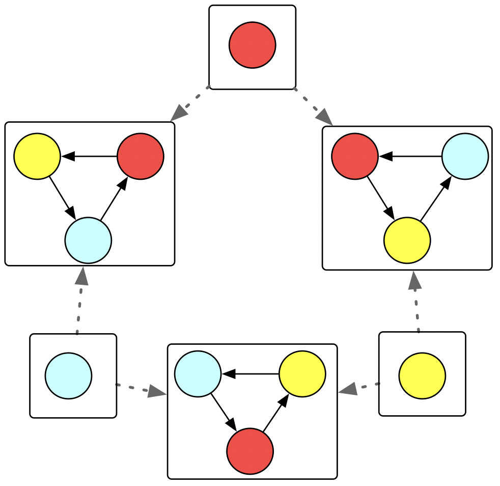

This is what the diagram represents with the building blocks substituted in. Although there’s a technical term for this, called a colimit, we informally call this gluing building blocks along shared boundaries (which are, in this case, those isolated vertices).

Structural mathematics allows us to have a good understanding of what this gluing process is even without knowing what is inside the bubbles and the junctions. We didn’t have to know much about the internal structure of a triangle or how it was constructed to do this - we simply stated how these existing things were related to each other, something external to the graph building blocks. We just declared what we wanted as a piece of data, rather than writing another piece of hacky code that will become someone else’s problem to debug down the line.

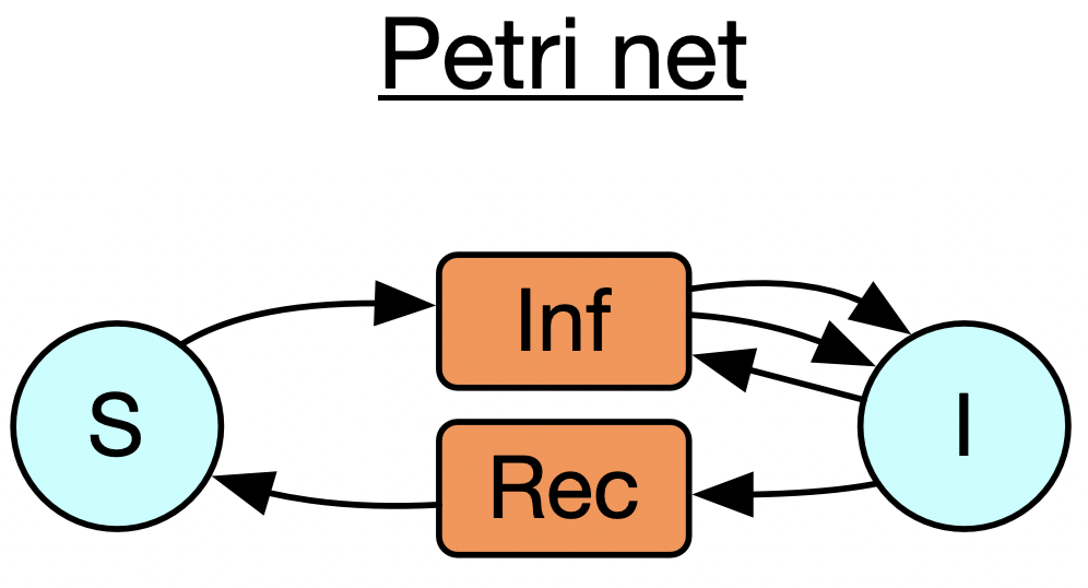
Abstraction: Petri nets

struct PetriNet
  S::Set{Symbol}
  T::Dict{Symbol, 
       Pair{Vector{Symbol},
            Vector{Symbol}
           }
     }
end

@present SchemaPetriNet(FreeSchema) begin 
  (S, T, I, O)::Ob
  is::Hom(I, S)
  os::Hom(O, S)
  it::Hom(I, T)
  ot::Hom(O, T)
end
@acset_type PetriNet(SchemaPetriNet)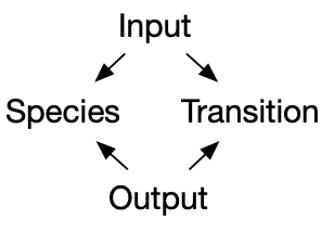

sis = PetriNet(Set([:S, :I]), 
               Dict(:inf => ([:S,:I] => [:I,:I]),
                    :rec => ([:I]    => [:S])))

function ODE(p::PetriNet, rates, init, time) end
function stochastic(p::PetriNet, rates, init, time) end

New problem expressed in terms of old problem.

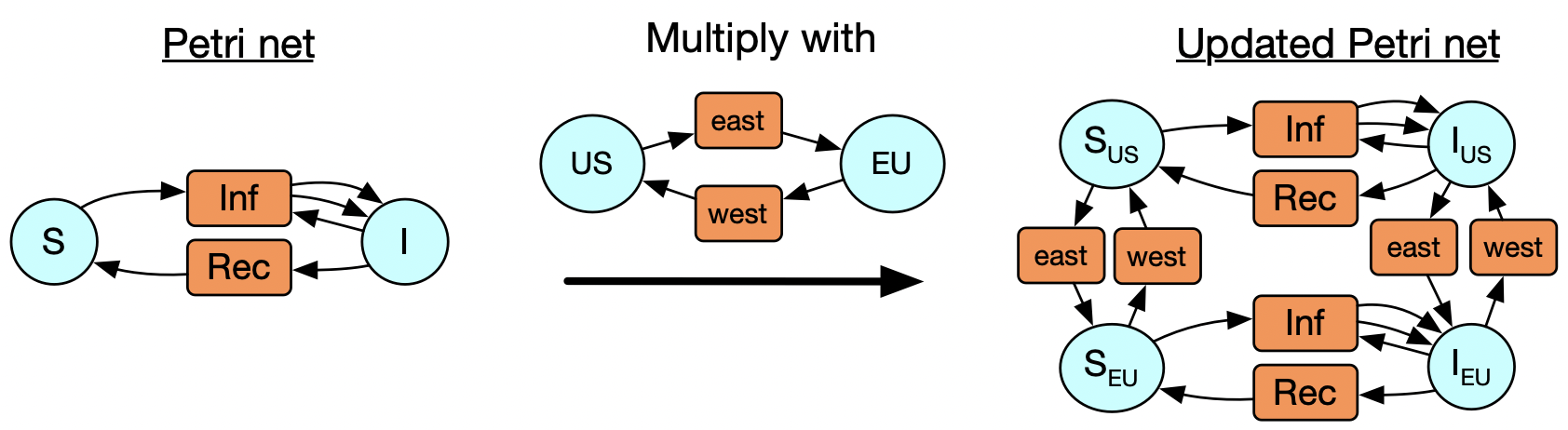
Next, I want to move onto Petri nets, which are a way of looking at bipartite graphs, where we interpret one of the vertex types, call them transitions, as hyperedges which have multiple inputs and multiple outputs. This is especially relevant to modeling epidemiology or supply chains or chemical reaction networks. It might be of interest that these can also be thought of as instances of a certain database schema, which means if we understand the basic structure of databases then we do not have to write much Petri-net-specific code at all.

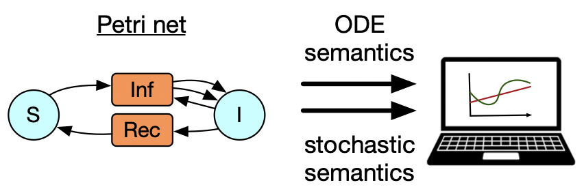
Let’s start with the example of a world where there are susceptible and infected people, and it takes a susceptible + an infected person to make two infected people, and the infected people can recover spontaneously too. This is just a specification of what sorts of transitions are possible without saying anything about their rates. There are two particular ways of taking a positive real number weight for each transition and obtaining a dynamical system: one of which is to create an ODE using mass-action kinetics (like in chemistry) and another is to do a stochastic simulation where you keep track of individual tokens living inside all of the blue circles and randomly trigger the transitions to fire. (…)

I’m going to talk about a new problem, but should first mention that the gluing problem from before is still relevant to petri nets. We can do the exact same AlgebraicJulia solution from before (flip back to previous slide) if we wanted without having to write any new code, whereas our two code-based solutions from before would have to be rewritten from scratch, something that feels very similar but still is completely different because these data structures look pretty different. But to keep things interesting let me talk about a different kind of abstraction reuse problem in the Petri net scenario.

Now consider that we may realize that, after running our simulation, that we should have made a distinction: what we thought was one homogenous group of susceptible people is better modeled by two US and a European populations, and likewise for infected people. It’s possible for someone to travel by plane and move from one of these populations to the other, too. We could express this itself as a Petri net with two states and two transitions, and only might we realize that our new model is really the multiplication of our starting Petri net with another one, in a sense that can be made precise. It would be nice to be able to declare that and be done with it, but first I’ll walk you through how we’d to do this in the old paradigm.

Multiplying: side-by-side comparison

prepend(pre) = s -> pre * "_" * s

US, EU, E, W = 
  prepend.(["US", "EU", "east", "west"])

function mult_EU(petri::PetriNet)
  res = PetriNet()
  for state in petri.S
    us = add_state!(res, US(state))
    eu = add_state!(res, EU(state))
    add_transition!(res, E(state), [us]=>[eu])
    add_transition!(res, W(state), [eu]=>[us])
  end
  for (T, (I, O)) in petri.T
    add_transition!(res, US(T), US.(I)=>US.(O))
    add_transition!(res, EU(T), EU.(I)=>EU.(O))
  end
  res
end

function multiply(r1::PetriNet, r2::PetriNet)
  res = PetriNet()
  for (s1, s2) in Iterators.product(r1.S, r2.S)
    add_state!(res, "$(s1)_$(s2)")
  end
  for rx1 in r1.T
    for s2 in r2.S
      add_transition!(res, rename_rxn(rx1, s2))
    end
  end
  for rx2 in r2.T
    for s1 in r1.S
      add_transition!(res, rename_rxn(rx2, s1))
    end
  end
  RxnNet(rs)
end

rename_rxn(rxn, species::Symbol) = # TODO

Our first approach is going to be a function which takes an arbitrary Petri net and ‘multiplies’ it with the EU petri net, i.e. for every state in the original Petri net, it creates a US and an EU version of it (and a corresponding travel transition in each direction). We then need a copy of the original transitions living in both the US and EU parts of the Petri net.

The second approach is more general but requires more work. It is going to multiply two arbitrary Petri nets, by first creating a species for every pair of species in the original, and then a transition for every pair of species and transition in the other Petri net.

Both of these require a lot of string name hacking, and this code completely breaks if we were to try to do something similar on a different data structure.

Multiplying: back to basics

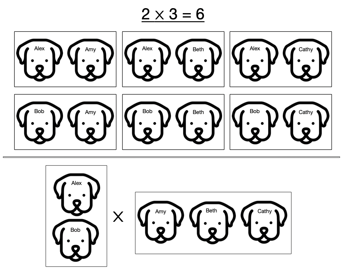
I want to explain why we are in some sense “multiplying” the two Petri nets. Let’s start off with our normal notion of multiplying numbers: take \(2 \times 3 = 6\). The essence of this is that we have two sets of things and multiplying is asking how many pairs there are where we take something from one set and something from the other. So here we have the male dogs Alex and Bob and the females Amy, Beth, and Cathy. And the fact that there are six possible pairings is what is expressed by \(2 \times 3 = 6\).

Multiplying: back to basics

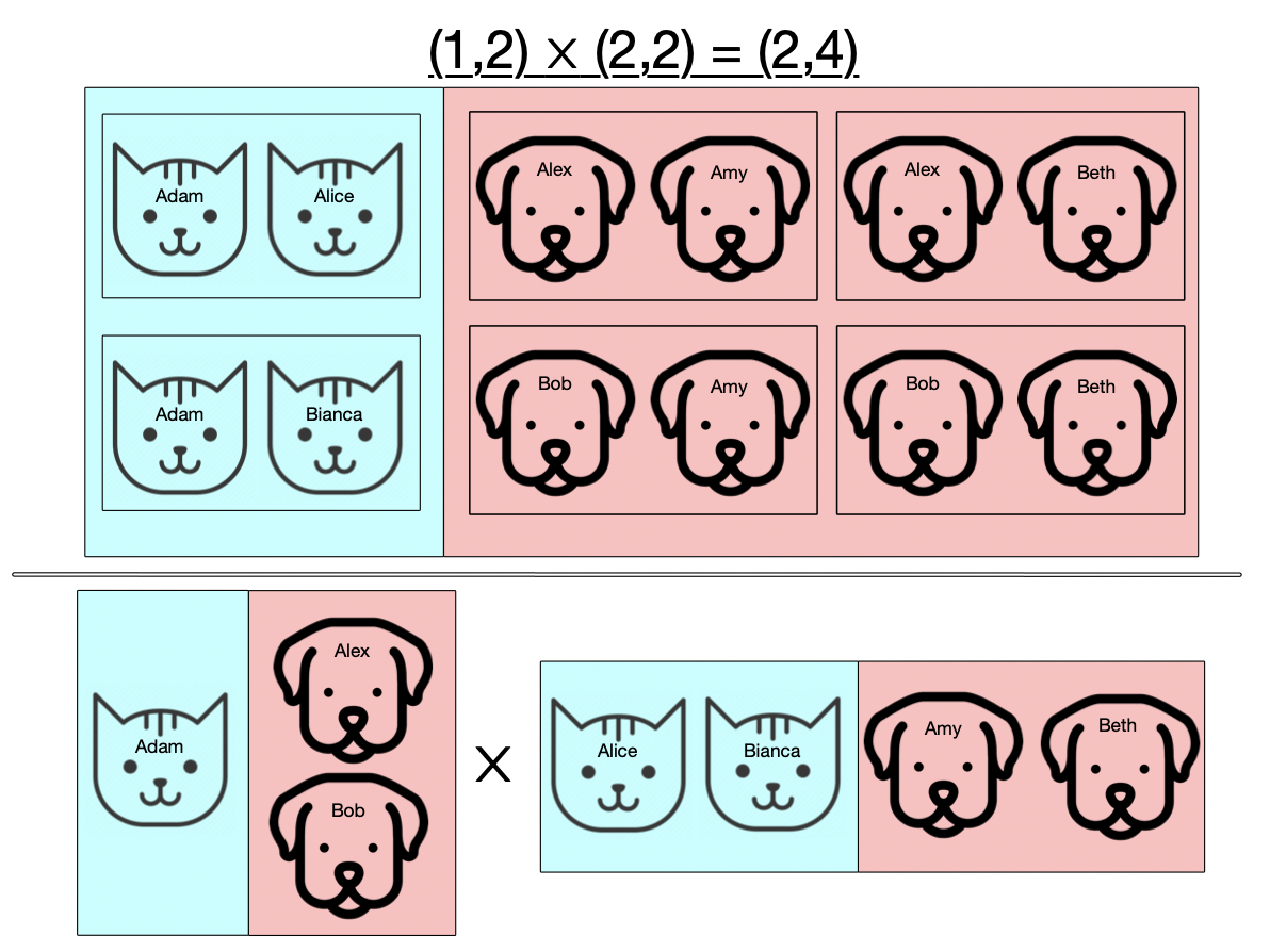
Now suppose our sets can have two kinds of things, say cats and dogs. When we take pairs of these, we’re only going to allow the ones which are of the same kind, so we won’t pair female cats with male dogs, for example.

Multiplying: back to basics

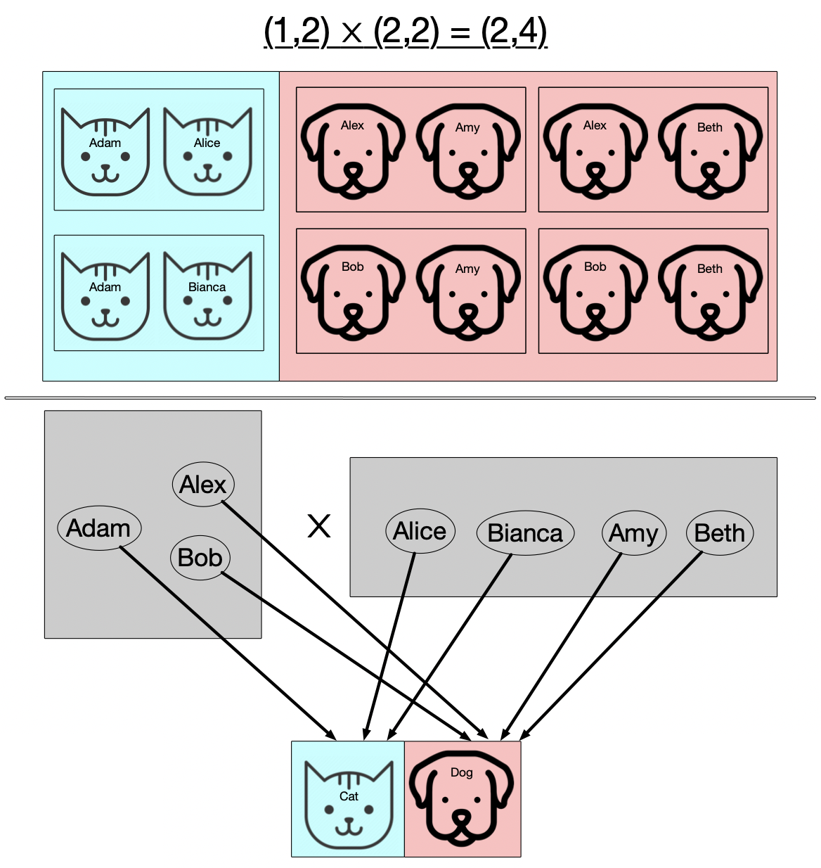
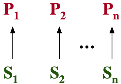
Now this slide presents the same information as the previous one, but rather than depicting the things we’re multiplying directly as two different kinds of things, we instead have at the bottom a common language of types of things (in this case, just cats and dogs) and our two sets have functions which assign to each thing what type of thing it is. This is the general form of multiplication that we’ll need in order to multiply our Petri nets.

Our generalized notion of gluing things together, did not rely on the internals of what we were gluing but just how they were externally related to each other (their relation to the boundary we glued them along). Here I hope you see the analogous thing happening for multiplicaiton: rather than multiplying these two sets based on what type of thing each element is in itself, we multiply the sets based on the external realtion of the two sets to some common set of types of things.

Multiplying: side-by-side comparison

prepend(pre) = s -> pre * "_" * s

US, EU, E, W = 
  prepend.(["US", "EU", "east", "west"])

function mult_EU(petri::PetriNet)
  res = PetriNet()
  for state in petri.S
    us = add_state!(res, US(state))
    eu = add_state!(res, EU(state))
    add_transition!(res, E(state), [us]=>[eu])
    add_transition!(res, W(state), [eu]=>[us])
  end
  for (T, (I, O)) in petri.T
    add_transition!(res, US(T), US.(I)=>US.(O))
    add_transition!(res, EU(T), EU.(I)=>EU.(O))
  end
  res
end

function multiply(r1::PetriNet, r2::PetriNet)
  res = PetriNet()
  for (s1, s2) in Iterators.product(r1.S, r2.S)
    add_state!(res, "$(s1)_$(s2)")
  end
  for rx1 in r1.T
    for s2 in r2.S
      add_transition!(res, rename_rxn(rx1, s2))
    end
  end
  for rx2 in r2.T
    for s1 in r1.S
      add_transition!(res, rename_rxn(rx2, s1))
    end
  end
  RxnNet(rs)
end

rename_rxn(rxn, species::Symbol) = # TODO

AlgebraicJulia

P_base = @acset PetriNet begin 
  S=1; T=2; I=2; O=2; is=1; os=1; it=1:2; ot=1:2 
end

# Label P1 and P2 transitions as green or orange
h1 = homomorphism(P1, P_base; init=...)
h2 = homomorphism(P2, P_base; init=...)

# Composition of old problems
US_EU_SIS = multiply(h1, h2)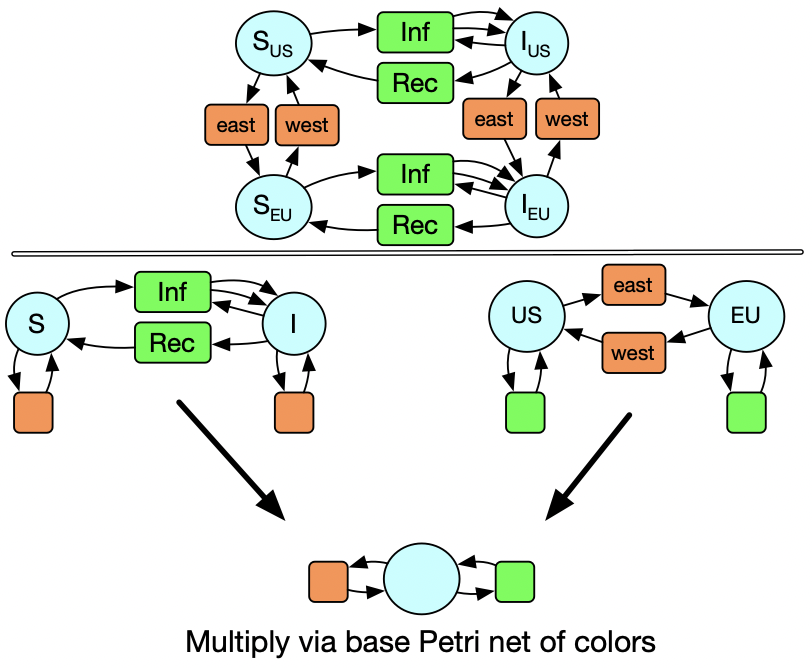

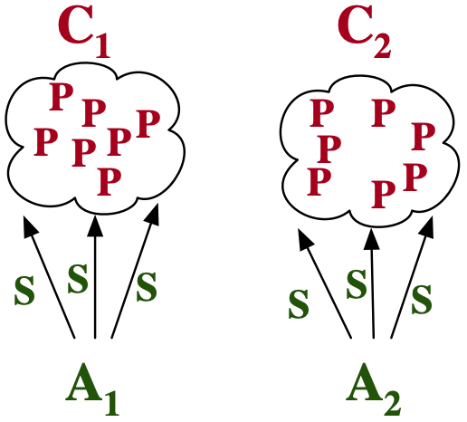
So instead of multiplying sets, we are multiplying Petri nets. We actually have a Petri net of colors. Here we see there is only one type of species and two types of transitions. The coloring of the circles and boxes of the SIS and US_EU models illustrates the data of these maps into the base Petri net of colors.

Multiplying: side-by-side comparison

prepend(pre) = s -> pre * "_" * s

US, EU, E, W = 
  prepend.(["US", "EU", "east", "west"])

function mult_EU(petri::PetriNet)
  res = PetriNet()
  for state in petri.S
    us = add_state!(res, US(state))
    eu = add_state!(res, EU(state))
    add_transition!(res, E(state), [us]=>[eu])
    add_transition!(res, W(state), [eu]=>[us])
  end
  for (T, (I, O)) in petri.T
    add_transition!(res, US(T), US.(I)=>US.(O))
    add_transition!(res, EU(T), EU.(I)=>EU.(O))
  end
  res
end

function multiply(r1::PetriNet, r2::PetriNet)
  res = PetriNet()
  for (s1, s2) in Iterators.product(r1.S, r2.S)
    add_state!(res, "$(s1)_$(s2)")
  end
  for rx1 in r1.T
    for s2 in r2.S
      add_transition!(res, rename_rxn(rx1, s2))
    end
  end
  for rx2 in r2.T
    for s1 in r1.S
      add_transition!(res, rename_rxn(rx2, s1))
    end
  end
  RxnNet(rs)
end

rename_rxn(rxn, species::Symbol) = # TODO

AlgebraicJulia

P_base = @acset PetriNet begin 
  S=1; T=2; I=2; O=2; is=1; os=1; it=1:2; ot=1:2 
end

# Label P1 and P2 transitions as green or orange
h1 = homomorphism(P1, P_base; init=...)
h2 = homomorphism(P2, P_base; init=...)

# Composition of old problems
US_EU_SIS = multiply(h1, h2)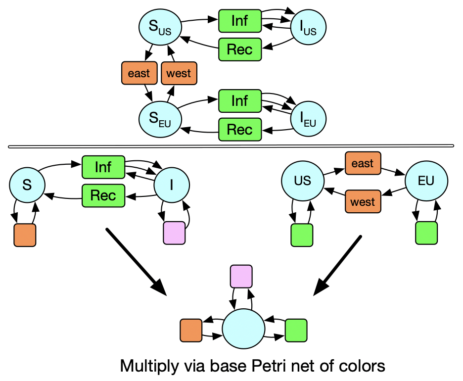

We might also think that it makes sense for susceptible people to be able to travel internationally but not sick people. A slight modification of this diagram is sufficient to allow us to still just declare how the two models are related and have the multiplication do the right thing.

Abstraction: Wiring diagrams

function goods_flow(steps::Int, initial::Vector, 
                    input::Function)
  output = []
  trade₁, trade₂ = initial
  for step in 1:steps
    trade₁, (trade₂, out) = [
      trader₁(input(step), trade₂),
      trader₂(trade₁)
    ]
    push!(output, out)
  end
  output
end

"""
A + B = C
±√(C) = (B, D) 

Find all integer solutions (A, D) up to `n`
"""
function solve_constraint(n::Int)
  filter(Iterators.product(0:n, 0:n)) do (A, D)
    B = -D
    C = A + B
    C == D^2
  end
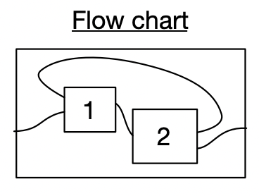
end

Here are two ways we might be doing something conceptually specified by the flowchart.

Abstraction: Wiring diagrams

New problem expressed in terms of old problem.

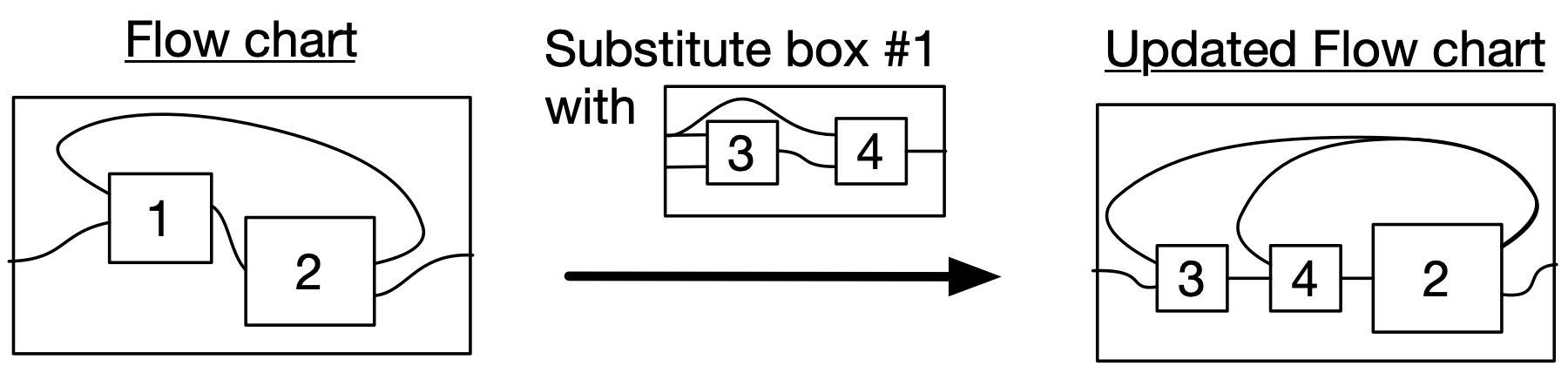
A wiring diagram substituion expresses that a process fits into another process as a subprocess. The subtitution is possible because this subprocess’ outer box matches the interface of this inner box.

Substituting: side-by-side comparison

function goods_flow(steps::Int, initial::Vector, 
                    input::Function)
  output = []
  trade₁, trade₂ = initial
  for step in 1:steps
    trade₁, (trade₂, out) = [
      trader₁(input(step), trade₂),
      trader₂(trade₁)
    ]
    push!(output, out)
  end
  output
end

\(\Rightarrow\)

function goods_flow(steps::Int, initial::Vector, 
                    input::Function)
  output = []
  trade₂, trade₃, trade₄ = initial
  for step in 1:steps
    trade₂, trade₃, (trade₄, out) = [ 
      trader₂(trade₃),
      trader₃(input(step), trade₂),
      trader₄(trade₃, trade₂),
    ]
    push!(output, out)
  end
  output
end

This is our process for updating the trading simulation with respect to this high-level change.

If we’d had a piece of code which solves the 3 4 system, we couldn’t re-use it.

Substituting: side-by-side comparison

"""
A + B = C
±√(C) = (B, D) 

Find all integer solutions (A, D) up to `n`
"""
function solve_constraint(n::Int)
  filter(Iterators.product(0:n, 0:n)) do (A, D)
    B = -D
    C = A + B
    C == D^2
  end
end

\(\Rightarrow\)

"""
A + B = C
C * B = D
±√(D) = (B, E) 

Find all integer solutions (A, E) up to `n`
"""
function solve_constraint(n::Int)
  filter(Iterators.product(0:n, 0:n)) do (A, E)
    B = -E
    C = A + B
    D = C * B 
    D == E^2
  end
end

This is our process for updating the equation solver with respect to this high-level change.

If we’d had a piece of code which solves the 3 4 system, we couldn’t re-use it.

Substituting: side-by-side comparison

sys₁ = Trader(2, 1, (x,y)-> ...)
sys₂ = Trader(1, 2, (x,)-> ...)
sys₃ = Trader(2, 1, (x,y)-> ...)
sys₄ = Trader(2, 1, (x,y)-> ...)

sys₁ = Relation(2, 1, (xs,ys)-> xs[1] + xs[2] == ys[1])
sys₂ = Relation(1, 2, (xs,ys)-> sqrt(xs[1]) == ys[1] 
                                && ys[1]== -ys[2])
sys₃ = sys₁
sys₄ = Relation(2, 1, (xs,ys)-> xs[1] * xs[2] == ys[1])

AlgebraicJulia

wd₁₂ = WiringDiagram([:A], [:A])
b1 = add_box!(wd₁₂, Box(:op₁, [:A, :D], [:C]))
b2 = add_box!(wd₁₂, Box(:op₂, [:C], [:D, :A]))
add_wires!(wd₁₂, Pair[
  (input_id(wd₁₂), 1) => (b1, 2),
  (b1, 1)          => (b2, 1),
  (b2, 1)          => (b1, 1),
  (b2, 2)          => (output_id(wd₁₂), 1)
])

model = oapply(wd₁₂,[sys₁,sys₂])
wd′ = ocompose(wd₁₂, 1, wd₃₄)
model′= oapply(wd′,[sys₂,sys₃,sys₄])

With AlgebraicJulia, rather than just having the flowchart be something that inspires us from the whiteboard to write some code, we reason about it as a piece of data. The code we would’ve written is constructed automatically by saying what goes in each box and having a mathematical understanding of what is in general required to go from saying what is in each box to saying what the outer box does.

Changing from one abstraction to another

New problem expressed in terms of old problem.

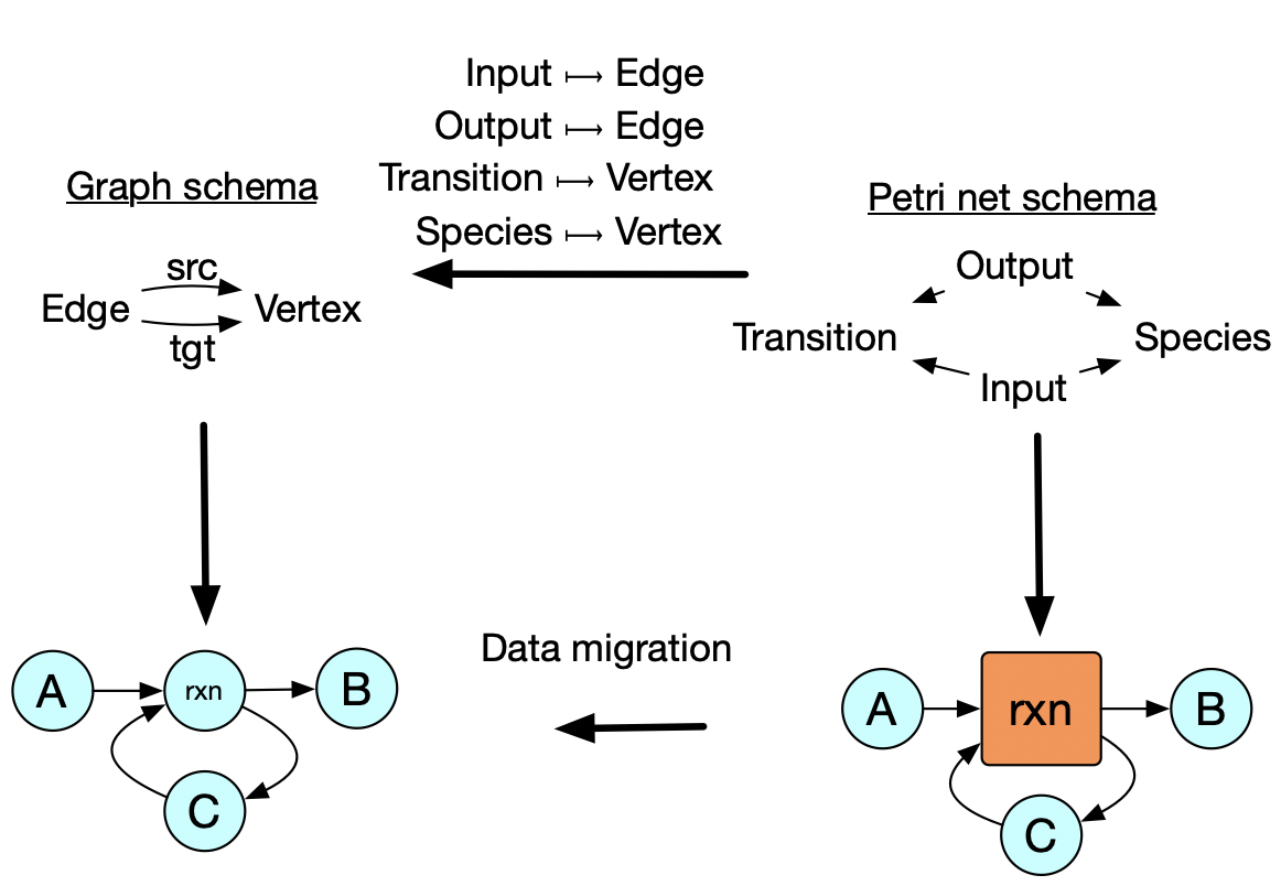
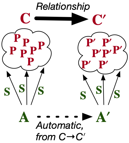
In addition to the previous examples which show re-use of abstractions within each of the three data types, this example shows how we can preserve an abstraction even when we change the data type: one might write a chemical reaction simulator that accepts Petri nets, but for other parts of one’s analysis one might not be working with general Petri nets. There are many algorithms and concepts that make sense for ordinary directed graphs that don’t make sense for Petri nets, so one ought work for as long as possible in the restricted setting with the knowledge that, at the end, one can identify graphs with a special kind of Petri net (i.e. those which have transitions with exactly one input and one output). What may be surprising is that this transformation process is completely automated, just given a simple relationship between the two database schemas at the top. Structural mathematics tells us how to specify the relationships between specifications such that implementations can be migrated from one to the other in a meaning-preserving way.

Changing from one abstraction to another

New problem expressed in terms of old problem.

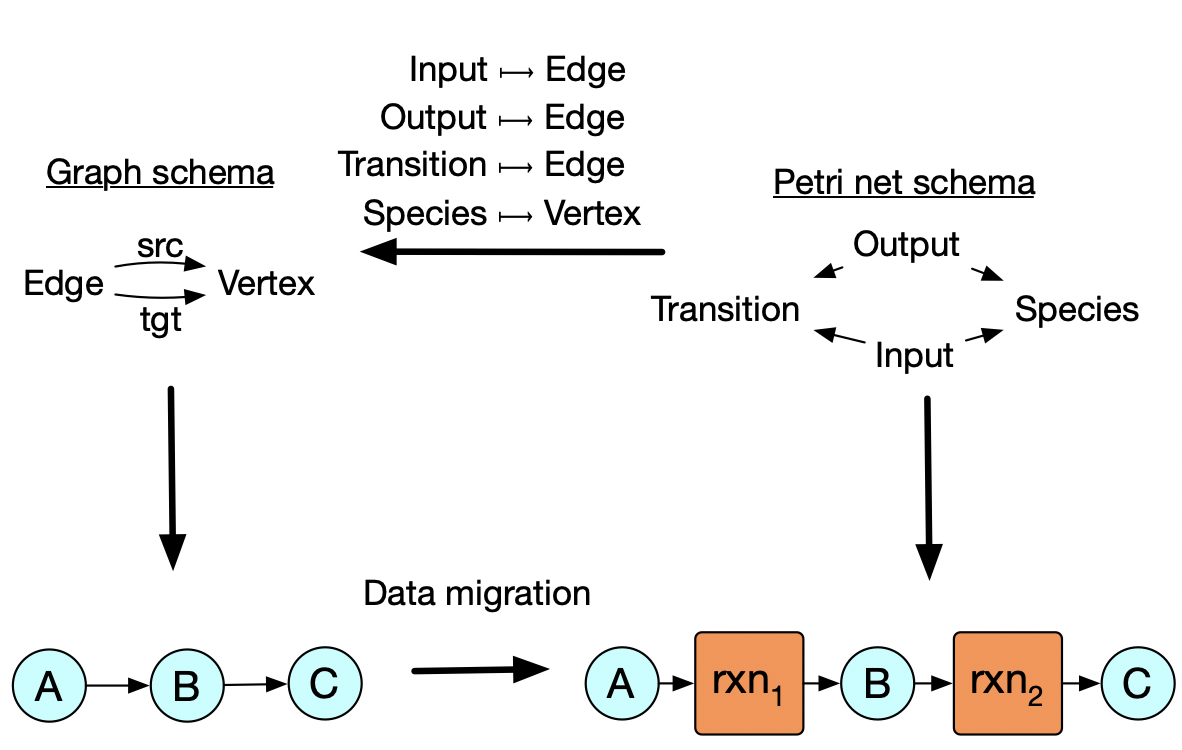
This high level data to relate the two schemas can be also used to move data in the other direction. So maybe what we need at the end of the day is a petri net, but we want to do our fancy graph algorithms with certain graphs and then convert them to Petri nets at the end.

Changing abstractions: side-by-side

"""Species and transitions are vertices.
   Inputs and outputs are edges."""
function petri_to_graph(p::PetriNet)
  grph = Graph()
  vs = Dict(s => add_vertex!(grph) for s in p.S)
  for (t, (i, o)) in pairs(p.T)
    t = add_vertex!(grph) 
    for eᵢ in i 
      add_edge!(grph, vs[eᵢ], t)
    end 
    for eₒ in o
      add_edge!(grph, t, vs[eₒ])
    end 
  end
  grph
end

"""
Vertices are species.
Edges are transitions with one input and
one output.
"""
function graph_to_petri(g::Graph)
  P = PetriNet()
  for i in G.vertices
    add_species(P, Symbol("v$i")) 
  end
  for (e, (s, t)) in enumerate(G.edges)
    add_transition(Symbol("e$e"),
                   [P.S[s]] => [P.S[t]])
  end
  P
end

AlgebraicJulia

F = FinFunctor(SchPetri, SchGraph; 
  init = (S => V, T => V, I => E, O => E))
my_graph = SigmaMigration(F, my_petri)

F = FinFunctor(SchPetri, SchGraph; 
  init = (S => V, T => E, I => E, O => E))
my_petri = DeltaMigration(F, my_graph)

Here we simply declare the relationship between the two schemas and say how we want to interpret it (the name of action which pushes data forward along the map is called sigma and the one which moves data the opposite direction is called delta).

Replacing code with data

Common theme: writing code vs declaring relationships between abstractions.

Problem	Julia solution	AlgebraicJulia solution
Different pieces of a model need to be glued together.	Write a script which does the gluing or modifies how pieces are constructed.	Declare how overlap relates to the building blocks. (colimits)
Different aspects of a model need to be combined / a distinction is needed.	Write a script which creates copies of one aspect for every part of the other aspect.	Declare how the different aspects interact with each other. (limits)
We want to integrate systems at different levels of granularity.	Refactor the original code to incorporate the more detailed subsystem.	Separate syntax/semantics. Declare how the part relates to the whole at syntax level. (operads)
We make a new assumption and want to migrate old knowledge into our new understanding.	Write a script to convert old data into updated data.	Declare how the new way of seeing the world (i.e. schema) is related to the old way. (data migration)

So to summarize these past toy examples, there are some very general kinds of ways that we recognize a problem has shifted and we wish to reuse our old abstractions towards the new problem. In any specific scenario, one can always write an ad hoc function or script to handle this, but once you do this time after time, these one-off solutions become unmaintainable spaghetti. This is in contrast to the eat-your-cake-and-have-it-too solution on the right, where we have general solutions which do not need to be rewritten for every new scenario that pops up. And the way these compose together is transparent.

Of course, it’s not magic, and this strategy isn’t immediately available whenever we dream up of a new domain. Structural mathematics shows us what structure to look for in a new domain that allows us to do these things, though it’s still a case-by-case process to take domain-expert’s knowledge and find this structure. In the next section I’m going to give a high level picture of how this works.

Why does it work?

Informal definition: a category is a bunch of things that are related to each other

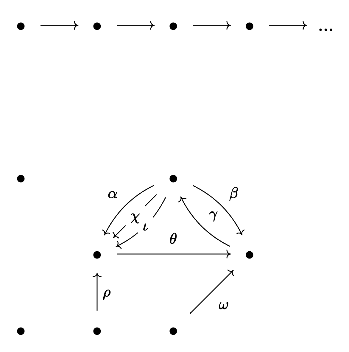
Key intuition: category theory is concerned with universal properties.

• These change something that we once thought of as a property of an object into a kind of relationship that object has towards related objects.

Goal of talk is not to communicate how category theory works at a technical level. This is why this is the only definition which will be featured in the talk. (…)

But it’s important to get an intuition for why it works to know it’s not magic. I think the philosophy of category theory, which encourages working with universal properties, is a good explanation. I’ll try to describe one example of the simplest universal property just to give you some intuition for how it works.

Example universal property: emptiness

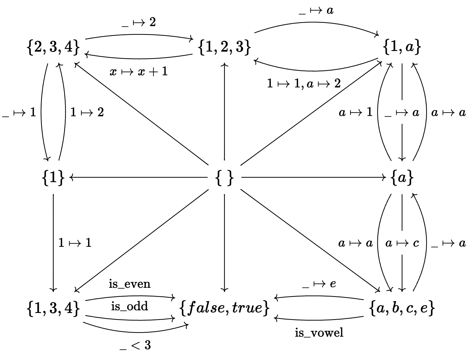
Consider mathematical sets which are related to each other via functions.

Definition in terms of internal properties

The empty set is the unique set which has no elements in it.

But if we we look at how the empty set relates to all the other sets, we’ll eventually notice something about these relations.

Definition in terms of external relationships (universal properties)

The empty set is the unique set which has exactly one function into every other set.

So if you were to tell a high schooler what an empty set is, this is a perfectly good definition. However, it doesn’t automatically generalize to telling us what an empty matrix is, or what an empty dynamical system or graph is. (…)

Example universal property: emptiness

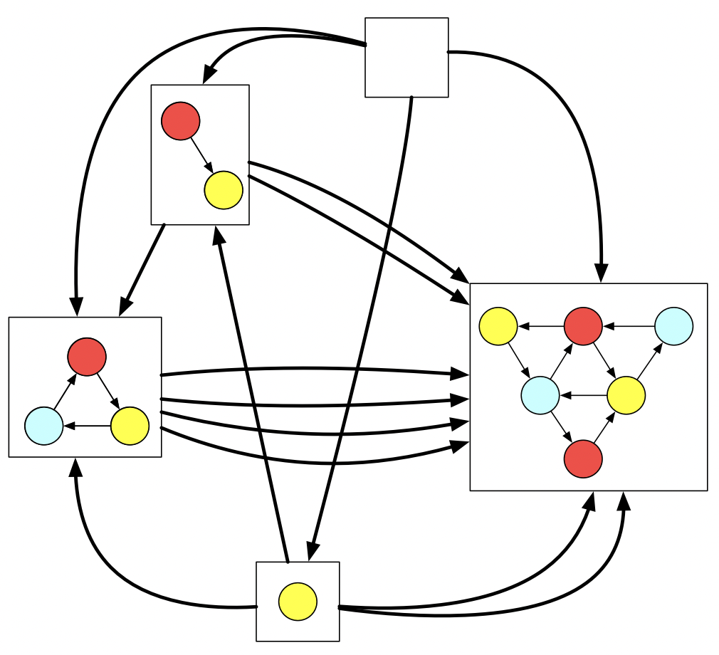
Consider colored graphs related to each other via vertex mappings which preserve color and edges.

Definition in terms of internal properties

The empty graph uniquely has no vertices nor edges in it.

But if we we look at how it relates to all the other graphs, we’ll eventually notice something characteristic.

Definition in terms of external relationships (universal properties)

The empty graph is the unique graph which has exactly one graph mapping into every other graph.

We can see that the yellow vertex lives within the triangle in one way but in the big triangle in two ways, etc. If I wanted to say why this is the empty graph, of course my first instinct would be to say “Just look at it! There are no vertices, no edges!”. But look that our same definition from earlier which says to look for the object which is related to every other object exactly once also applies here.

Universal properties and generalizable abstractions

Category theory enforces good conceptual hygeine - one isn’t allowed to depend on “implementation details” of the things which feature in its definitions.

This underlies the ability of models built in AlgebraicJulia to be extended and generalized without requiring messy code refactor.

When you structure your code around these definitions, you inherit this kind of generalizability.

Takeaways

CT is useful for the same reason interfaces are generally useful.

In particular, CT provides generalized¹ notions of:

• multiplication / multidimensionality
• adding things side-by-side
• gluing things along a common boundary
• looking for a pattern
• find-and-replace a pattern
• parallel vs sequential processes

• Mad Libs style filling in of wildcards
• Zero and One
• “Open” systems
• Subsystems
• Enforcing equations
• Symmetry

These abstractions all fit very nicely with each other:

• conceptually built out of basic ideas of limits, colimits, and morphisms.

We can use them to replace a large amount of our code with high level, conceptual data.

I hope to have shown that just a few basic concepts in category theory, in particular morphisms, limits, and colimits, are a very versatile vocabulary of good abstractions. Various combinations of these are sufficient to capture all of the diverse kinds of activities you see up here in a very generic way that can be specialized to your domain once you view it categorically.

1. Defined by universal properties.

About the Topos Institute

Mission: to shape technology for public benefit by advancing sciences of connection and integration.

Three pillars of our work, from theory to practice to social impact:

1. Collaborative modeling in science and engineering
2. Collective intelligence, including theories of systems and interaction
3. Research ethics

• Physics simulations (PDEs) with Decapodes.jl
• Reaction networks with AlgebraicPetri.jl
• Epidemiological modeling with StockFlow.jl
• Agent-based modeling with AlgebraicRewriting.jl
• Interactive GUIs with Semagrams

• Vision: topos.institute
• Research: topos.site
• Blog: topos.site/blog

…

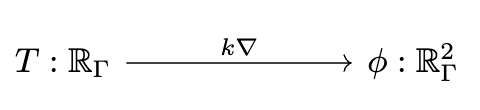
Decapodes.jl: multiphysics modeling

"""Define the multiphysics"""
Diffusion = @decapode DiffusionQuantities begin
  C::Form0{X}
  ϕ::Form1{X}
  ϕ == k(d₀{X}(C))   # Fick's first law
end
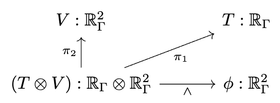
Advection = @decapode DiffusionQuantities begin
  C::Form0{X}
  (V, ϕ)::Form1{X}
  ϕ == ∧₀₁{X}(C,V)
end
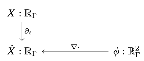
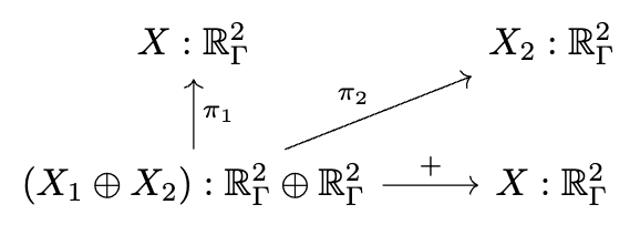
Superposition = @decapode DiffusionQuantities begin
  (C, Ċ)::Form0{X}
  (ϕ, ϕ₁, ϕ₂)::Form1{X}
  ϕ == ϕ₁ + ϕ₂
  Ċ == ⋆₀⁻¹{X}(dual_d₁{X}(⋆₁{X}(ϕ)))
  ∂ₜ{Form0{X}}(C) == Ċ
end
compose_diff_adv = @relation (C, V) begin
  diffusion(C, ϕ₁)
  advection(C, ϕ₂, V)
  superposition(ϕ₁, ϕ₂, ϕ, C)
end

"""Geometry"""
mesh = loadmesh(Torus_30x10()) 

"""Assign semantics to operators"""
funcs = sym2func(mesh)
funcs[:k] = Dict(:operator => 0.05 * I(ne(mesh)), 
  :type => MatrixFunc())
funcs[:⋆₁] = Dict(:operator => ⋆(Val{1}, mesh, 
  hodge=DiagonalHodge()), :type => MatrixFunc());
funcs[:∧₀₁] = Dict(:operator => (r, c, v) -> r .= 
  ∧(Tuple{0,1}, mesh, c, v), :type => InPlaceFunc())

Extending what I’ve said so far to the design of simulators amounts to the following:

• simulations should be compiled to code rather than written in code
• This is because we can do high level conceptual programming (e.g. limits and colimits) when we are working with data, whereas representing our simulation via code will forever condemn us to having every conceptual update require a painstaking manual code update that could be very challenging.

When we work at the low level of code, introducing a simple mathematical idea (for example adding a gravitation force) forces us to remind ourself of all the implementation details - there could be a cascade of changes required.

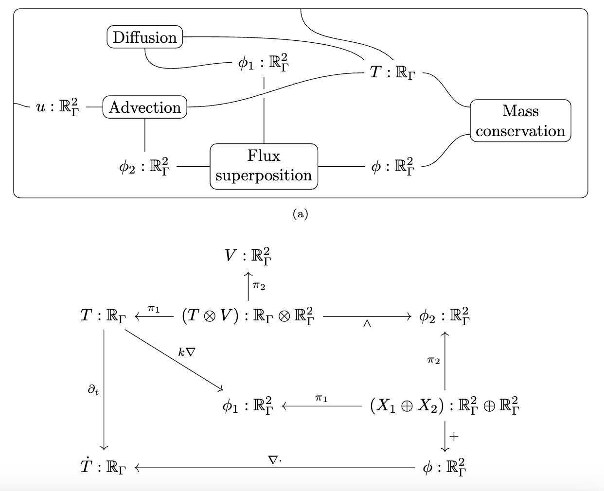
I can only briefly gesture at the work done by some of my colleagues in a compositional language for multiphysics. The idea is that there is a graphical language for specifying equations which rigorously corresponds to things like Fick’s law of diffusion and conservation of mass. This is just like how our Petri Nets were a nice graphical language which could rigorously be interpreted as Chemical Reaction Networks and how spans of models can be rigorously interpreted as models glued along an overlap.

There is some interesting math behind how this works which I won’t be able to get into, involving something called the “discrete exterior calculus”, but from a user perspective you can see us declaring each of these small diagrams and then composing them together along shared variables into a multi-physics.

We then need to give a computational semantics by associating linear operators with some of the primitive building blocks, such as “multiplication by k” being 0.05 times the identity matrix.

We decoupled the high level physics from the geometry and the implementation.

Decapodes.jl: simulation

Resources

• Papers and talks: algebraicjulia.org
  • Computational chemistry database integration
  • Epidemiology and gene regulatory networks
  • Chemical reaction network model space exploration
• Blog posts: algebraicjulia.org/blog and topos.site/blog
  • Introductory posts on C-Sets
  • What is a scientific model?
  • Building dynamical systems compositionally
• Code: github.com/AlgebraicJulia
  • DECAPODES.jl
  • AlgebraicPetri.jl
  • AlgebraicRewriting.jl

If you want to follow up on any the ideas in this talk, we have lots of papers, a couple of which I point out here to be potentially of interest to scientists. We also write blog posts intended to be more accessible and conversational, and I highlight a few here. Our code is always open source and we’re delighted to see it getting used.

Hidden slide: this slide intentionally left blank

You’re not supposed to be here.

Hidden slide: Why Category Theory?

Focuses on relationships between things without talking about the things themselves.

Invented in the 1940’s to connect different branches of math.

A category consists of objects and morphisms (arrows).

• We don’t need to know anything about the objects.
• Compose \(A \rightarrow B\) and \(B \rightarrow C\) to get \(A \rightarrow C\).
• Like a graph, but we care about paths, not edges.

CT studies certain shapes of combinations of arrows.

• These can be local shapes, e.g. a span:    \(\huge \cdot \leftarrow \cdot \rightarrow \cdot\)
  
  
• These can be global, e.g. an initial object: \(\huge \boxed{\cdot \rightarrow \cdot\rightarrow \cdot \rightarrow \dots}\)

Let me introduce just enough about CT to explain how it could, in principle, be useful. [read slide]

Hidden slide: Applied Category Theory?

Compare to interfaces in computer science:

• declare that some collection of things are related in a particular way without saying what they are.

interface Queue{A}

size(q:Queue) -> Int 
empty(q:Queue) -> Bool 
put(q:Queue, a:A) -> ()
get(q:Queue) -> A 

In some sense a category is just a particular interface.

interface Category{Ob,Arr}

dom(a:Arr) -> Ob 
codom(a:Arr) -> Ob 
compose(a:Arr, b::Arr) -> Arr 
id(o:Ob) -> Arr

• Category of sets and functions
• Category of sets and subsets
• Category of \(\mathbb{Z}\) and \(\leq\)
• Category of categories and functors

• Category of chemical reaction networks
• Category of chemical structures
• Category of datasets
• Category of datatypes and programs

CT is also the study of interfaces in general. It knows which are good ones.

Let me try to connect this to a computer science concept you may be familiar with. In computer science you might declare an interface without caring how its specifically implemented. Programmers quickly learn that this kind of abstraction is really useful because your code can be much less brittle when it doesn’t make assumptions about the intrinsic nature of the things it interacts with: for example you start out with a linked-list implementation of a queue, but later you learn you need to switch to a vector implementation for performance reasons. None of your code had to break.

. . .

If you want to know how something abstract like category theory can be useful, first think of it as an interface for which mathematicians have been writing code for over the last century. All you need to do is show how chemical reaction networks implement the interface of a category and suddenly you have access to a rich library of questions to ask about your domain (e.g. what does a span or initial object correspond to?) and furthermore there is a formalism to relate different categories to each other, so you can make connections between different domains explicit.

. . .

The last thing I’ll say on this topic is that a category codifies caring about how things relate to each other without looking at the things themselves. So it is also an opinionated source of what are good interfaces.