Scientific and software engineering examples of applied category theory

Kris Brown - Topos Seminar


(press s for speaker notes)

6/5/23

Abstraction

$$

$$

It’s straightforward to write a make_shape function that abstracts the functions which produce these various shapes, perhaps taking an integer parameter and making the regular polygon with that many sides.

Separately, we make a different abstraction for allowing us to talk about different colors in a uniform way, for example, a class which takes Red Green Blue values and is interpreted as the corresponding color.

When we take these to be primitive building blocks, it’s natural to want to combine them together in these various ways. Conceptually, it’s very straightforward to specify how these building blocks should fit together, but in practice it is never as straightforward - programs don’t naturally fit together neatly in a high-level way. It turns out that we will likely have to dig deep into the implementation details of the make_shape function to make it interoperable with make_color (e.g. adding an extra parameter).

This is the problem we’re trying to solve: how do we design our abstractions to be extensible, to safeguard ourselves against future problems that we’ll later discover we want to solve?

The status quo

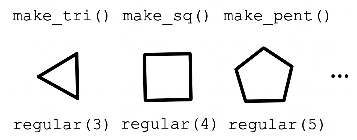
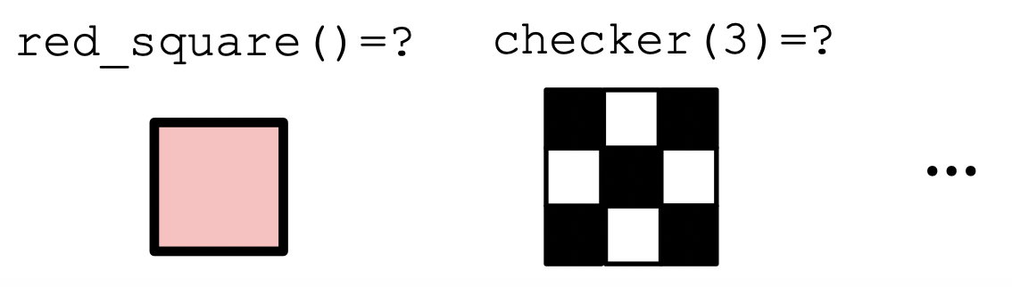
Abstraction is something all programmers are familiar with.

• There are pros and cons to it. Cons follow when abstractions are ad hoc.
• E.g. they don’t fit well together, difficult to modify, unintelligible to peers

Category theory offers abstractions that fit well together.

• Scientific workflow can be improved to be conceptual, not manual, programming.

I want to start with the topic of abstraction. If you’ve programmed before, you are familiar with having problems like “draw a triangle” and then “draw a square” so you write a function which takes a number, such as 5, and draws a pentagon. So we’ve abstracted away problem with a function, or a script, or a class. Maybe we also have a problem of rendering red, then blue, so you write a function to do that, and then we have a
Abstraction is very good for reducing tedium, but it’s very easy to get trapped by earlier abstractions one has made. They both become more of a hinderance when your problems unexpectedly change, and furthermore they’re unintelligible spaghetti to any collaborators looking at your code.

I hope to pique your interest in Category Theory, which is a branch of math which is a study of abstraction and provides abstractions which do fit will together and can be extended. I’ll claim that this helps you write better code that’s both abstract and less restrictive.

. . .

I’m now trying to visually depict the current status quo on the bottom. The scientist has a concept they’re trying to make computational. So they can start on the whiteboard and then, separately, try to then make a program that faithfully captures that concept. Sometimes it’s easier to encode the problem into the format of a standard solver (e.g. an ODE equation solver) and then the rest is automatic (these drawings will indicated dotted lines as the things that are done automatically). When we need to update our conceptual understanding, as happens often in science, we either have to go through our old code and fix what breaks or, as is often easier than that, start over from scratch.

So due to the gap overall this status quo is laborious, error-prone, and costly to maintain and evolve, especially for large models.

A better quo

⋅⋅⋅⋅⋅⋅⋅⋅⋅⋅⋅⋅⋅⋅⋅⋅⋅⋅⋅⋅⋅⋅⋅⋅⋅⋅⋅⋅⋅⋅⋅⋅⋅⋅⋅⋅⋅⋅⋅⋅⋅⋅⋅⋅⋅⋅⋅⋅⋅⋅⋅⋅⋅⋅⋅⋅⋅⋅⋅⋅⋅⋅⋅⋅⋅⋅⋅⋅⋅⋅⋅⋅⋅⋅⋅⋅⋅⋅⋅⋅⋅⋅⋅⋅⋅⋅⋅⋅⋅⋅⋅⋅⋅⋅⋅⋅⋅⋅⋅⋅⋅⋅⋅⋅⋅⋅⋅⋅⋅

In this proposed workflow, we reduce problems by conceptually breaking them down. Here our two ‘manual’ labor tasks are

1. to explicitly represent the composition patterns, and
2. to explicitly declare our concepts in a mathematical framework which we can assign a computational semantics to.

CT plays the role of a good language for declaring how things compose together and for assigning semantics. With that manual labor done, we obtain an automatic (shown by dotted line) way of obtaining a simulator for the whole concept.

It’ll become clear during the talk what I mean when I distinguish “model as data” and “model as code”.

. . .

The paradigm I’ll show also addresses this problem of updating one’s model. If we explicitly represent our model updates as data, we can automatically update our infrastrastructure to work with the new conceptual model.

Why Category Theory?

Focuses on relationships between things without talking about the things themselves.

Invented in the 1940’s to connect different branches of math.

A category consists of objects and morphisms (arrows).

• We don’t need to know anything about the objects.
• Compose \(A \rightarrow B\) and \(B \rightarrow C\) to get \(A \rightarrow C\).
• Like a graph, but we care about paths, not edges.

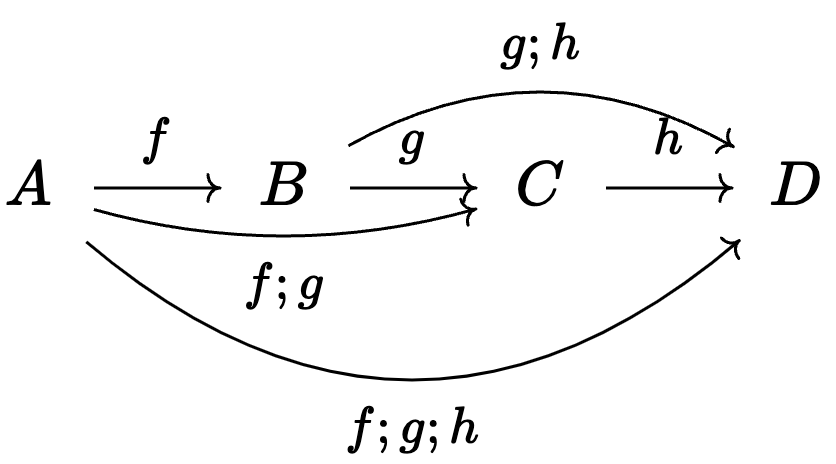
CT studies certain shapes of combinations of arrows.

• These can be local shapes, e.g. a span:    \(\huge \cdot \leftarrow \cdot \rightarrow \cdot\)
  
  
• These can be global, e.g. an initial object: \(\huge \boxed{\cdot \rightarrow \cdot\rightarrow \cdot \rightarrow \dots}\)

Let me introduce just enough about CT to explain how it could, in principle, be useful. [read slide]

Applied Category Theory?

Compare to interfaces in computer science:

• declare that some collection of things are related in a particular way without saying what they are.

interface Queue{A}

size(q:Queue) -> Int 
empty(q:Queue) -> Bool 
put(q:Queue, a:A) -> ()
get(q:Queue) -> A 

In some sense a category is just a particular interface.

interface Category{Ob,Arr}

dom(a:Arr) -> Ob 
codom(a:Arr) -> Ob 
compose(a:Arr, b::Arr) -> Arr 
id(o:Ob) -> Arr

• Category of sets and functions
• Category of sets and subsets
• Category of \(\mathbb{Z}\) and \(\leq\)
• Category of categories and functors

• Category of chemical reaction networks
• Category of chemical structures
• Category of datasets
• Category of datatypes and programs

CT is also the study of interfaces in general. It knows which are good ones.

Let me try to connect this to a computer science concept you may be familiar with. In computer science you might declare an interface without caring how its specifically implemented. Programmers quickly learn that this kind of abstraction is really useful because your code can be much less brittle when it doesn’t make assumptions about the intrinsic nature of the things it interacts with: for example you start out with a linked-list implementation of a queue, but later you learn you need to switch to a vector implementation for performance reasons. None of your code had to break.

. . .

If you want to know how something abstract like category theory can be useful, first think of it as an interface for which mathematicians have been writing code for over the last century. All you need to do is show how chemical reaction networks implement the interface of a category and suddenly you have access to a rich library of questions to ask about your domain (e.g. what does a span or initial object correspond to?) and furthermore there is a formalism to relate different categories to each other, so you can make connections between different domains explicit.

. . .

The last thing I’ll say on this topic is that a category codifies caring about how things relate to each other without looking at the things themselves. So it is also an opinionated source of what are good interfaces.

Outline

1. 🗄️ Data
   • CT: C-Sets, Homomorphisms, Data migration
   • Examples: Computational chemistry simulation generated data

2. 💭 Models
   • CT: Colimits, Limits
   • Examples: COVID models, Chemical Reaction Networks
3. 📈 Simulation
   • CT: Functors, DWDs, rewriting
   • Examples: Multiphysics PDEs, Agent-based models

Ok with those preliminaries, let me try to talk at a high level about different ways you could represent data, models, and simulations. We’ll start with talk of representing data.

🗄️. DFT simulations

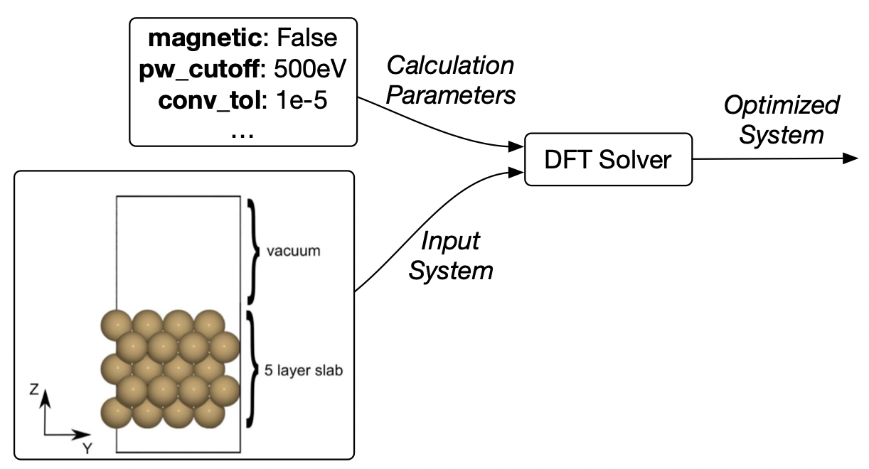
A simulation has the following data

I want to start incredibly concrete here. The scenario is that we have lots of simulations to run (this is from my phd). We want to vary some things, holding others fixed, and gain an insight.

The actual particulars of the data aren’t relevant to what’s conceptually important, but let me give a small amount of context anyway. We are doing simulations of chemical systems, which we represent with little boxes called unit cells which have atoms at various coordinates inside. We sometimes consider the edges of the box to be “periodic”, meaning we treat as if there are an infinite number of copies in all three dimensions. In the case of modeling a 2D surface such as the one shown here, we only want periodicity in the X and Y dimensions. We throw this into a density functional theory solver, or DFT, and depending on what calculation parameters we also feed it, we get various results in the form of optimized positions of atoms.

🗄️. Storing the data of lots of simulations

simulations
 |-bulk
 | |-magnetic
 | | |- Fe
 | | | |-pw_500/
 | | | |-pw_600/
 | | | |-pw_700/
 | |-nonmagnetic
 | | |- Al
 | | | |-pw_500/
 | | | |-pw_700/
 |-surface
 | |-...
 |-random
 | |- Ni lattice constant/
 | |- OH adsorbate interaction/

Problem

• Structure is not made explicit (unconstrained)
• It’s the wrong structure
  • arbitrary order on parameters
  • duplication of work

Instead, assemble the simulations into a big list and deduce experiments:

class Simulation():
  def __init__(self, calc: Calculator, sys: System):
  def write_input(self, pth: str):
  def read_input(pth: str) -> Simulation:
class Calculator():
  def __init__(self, params: Dict[str, Any]):
class System():
  def __init__(self, cell:Cell, atoms:List[Atom]):
class Cell():
  def __init__(self, dims:np.ndarray, pbc=Tuple[Bool,Bool,Bool]):
class Atom(Species):
  def __init__(self, elem: str,x:float,y:float,z:float):

Problem

• Inefficient/tedious querying
• Inefficient/tedious serialization
• Fragile infrastructure

A natural thing to do is to structure our filesystem around these experiments that we run. I won’t say much about this other than it’s not good - it’s what we first reach for because it’s so flexible, but the computer can’t guide us in doing things systematically, plus a tree structure is just the wrong abstraction for this shape of data.

. . .

A better model of the reality of our collection of experiments is that we just have a big list of them. We can make a data structure to characterize a simulation, and this object should be able to read/write to anywhere in the filesystem. When we’re doing analysis, we can load up all of the experiments into a list of Sims. The object oriented paradigm is an improvement because it makes the structure of our data explicit, but we need to always write custom code for each new question we want to ask about the data, in addition to writing code which stores the data, plus it’s very easy to write painfully slow code. And if our structure changes at any point, all of that custom code we wrote is liable to break. Unlike a tech company, scientists don’t have an army of software engineers to do this kind of tedium.

🗄️. An improvement: databases

Relational databases

• Each has a schema of entities, foreign keys, and attributes.
• These allow one to model things, relationships, and properties.
• A database instance has:
  • a table for each entity
    
  • a column for each FK+Attr
• Instances be efficiently queried using SQL language.

Example instance

Databases are a technology that address the issue of storing large amounts of data efficiently, across a wide range of data structures, while allowing for efficient retrieval of information. What kind of data structures are representable? Well we have to pick a schema, which is a collection of objects and arrows between them (my phrasing hints that we can view the schema as a category). These are the objects and relationships of the thing you a representing, and in database lingo they are tables and foreign keys.

. . .

Here is an example instance on this schema which attempts to model the data that goes into quantum chemistry calculations. (note: I’ve omitted the attributes in the schema). There are two simulations here, each with a distinct Calc but sharing the same system, which itself has an iron atom and two chromium atoms.

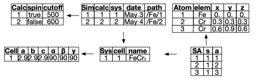
🗄️. Another improvement: C-Sets / ACSets

Problem

SQL solves the issue of querying and storage of data. But what do we do when we need to do more?

We must convert back from the database back into the custom data type, dealing with all of the problems associated with that.

A \(\mathsf{C}\)-set has the same information as a database without attributes.

Attributed \(\mathsf{C}\)-sets (ACSets) have the same information as ordinary relational databases.

Unlike databases, we understand ACSets as living in a category which supplies many interesting and useful things to do with database that we would otherwise not think to do.

The majority of this talk will emphasize the sorts of things one can do with this perspective.

Example ACSet

🗄️. Head-to-head comparison

# File System
simulations/
 |-bulk/
 | |-magnetic/
 | | |- Fe/
 | | | |-pw_500/
 | | | |-pw_600/
 | | |- ...
 | |-nonmagnetic/
 | | |- Al/
 | | | |-pw_500/
 | | | |-pw_700/
 | | |- ...
 |-surface/
 | |-magnetic/
 | |- Au/
 | | |-pw_500/
 | |...

# Python
class Atom():
  def __init__(self, elem,x,y,z):
  def __eq__(self, other):
class Cell():
  def __init__(self, dims, pbc):
  def __eq__(self, other):
class System():
  def __init__(self, cell, atoms):
  def __eq__(self, other):
class Calculator():
  def __init__(self, params):
  def __eq__(self, other):
class Sim():
  def __init__(self, calc, sys):
  def __eq__(self, other):
  def write_input(self, pth: str):
  def read_input(pth: str) -> Sim:

# AlgebraicJulia
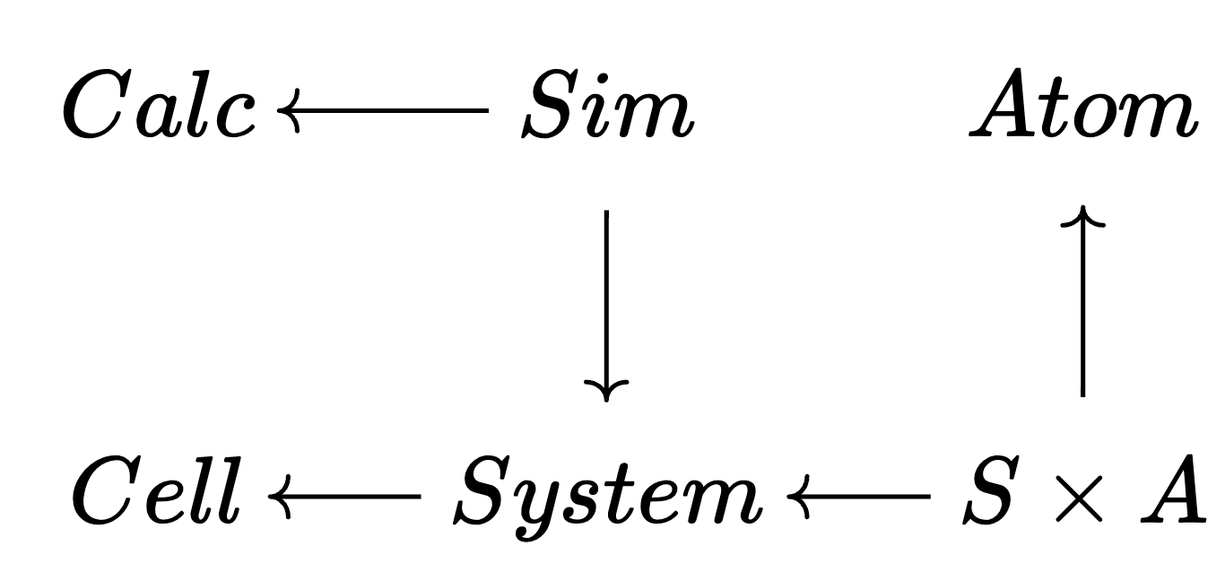
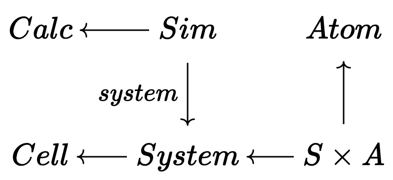
@present Simulations begin 
  (Atom,S_A,Cell,System,Sim,Calc) :: Ob
  (String, Float, Int) :: AttrType

  calc     :: Hom(Sim, Calc)
  system   :: Hom(Sim, System)
  cell     :: Hom(System, Cell)
  s_system :: Hom(S_A, System)
  s_atom   :: Hom(S_A, Atom)

  pw      :: Attr(Calc, Float)
  xc      :: Attr(Calc, String)
  (x,y,z) :: Attr(Atom, Float)
  elem    :: Attr(Atom, Int)
end

Find pairs of simulations with the same calculator and cell but different atomic configurations.

# Python
CHEM_LEVEL = 3
"""Put paths into buckets. Same bucket if 
their path (*ignoring* the 3rd folder name, 
i.e. chemical structure) is the same."""
def find_pairs(sim_path_root):
 EQcalc = defaultdict(list)
 for p in get_all_paths(sim_path_root)
  # e.g. p=["bulk","mag","Fe","pw_500",...]
  # pth_no_chem=["bulk","mag","pw_500",...]
  pth_no_chem = p[:CHEM_LEVEL]+p[CHEM_LEVEL+1:]
  bucket = (get_calc(p), pth_no_chem)
  EQcalc[bucket].append(p)
 end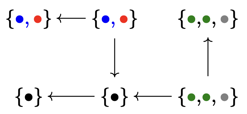
 return EqCalcCell.values()

# Python
def find_pairs(sims:List[Sim]):
  res = []
  for s1 in sims:
    for s2 in sims:
      if s1 != s2:
        if s1.calc == s2.calc:
          if s1.sys.cell == s2.sys.cell:
            res.append((s1,s2))
  return res 

-- SQL
SELECT S1.path, S2.path
  FROM Sim AS S1 JOIN Sim AS S2
  JOIN System AS Y1 ON S1.system = Y1.id
  JOIN System AS Y2 ON S2.system = Y2.id
WHERE S1.calc == S2.calc 
  AND Y1.cell == Y2.cell AND S1.id != S2.id 

# AlgebraicJulia
Q = @colim_repr Simulations begin 
  (s1, s2)::Sim 
  calc(s1) == calc(s2)
  cell(system(s1)) == cell(system(s2))
end
homomorphisms(Q, my_sim; monic=true)

So we have all three representations of the data side by side. On right is the AlgebraicJulia representation of this schema. Now I present you a scenario: you’ve run lots of calculations and the PI asks you: “I don’t know when you’re running the same parameters for different systems. Can show me all the pairs of calculations you’ve done that have the same parameters and the same cell but have different chemical compositions?” How will each of these three representations deal with this?

. . .

In the path-based representation of our data, this is tricky. In some sense, the “calculator” is identified by the path, except for the levels of the directory which characterize which system we are computing. This code is assuming level 3 of the hierarchy corresponds to choice of chemical composition, so it takes the directory information and lumps together all the paths which are the same, ignoring the third element. Then we need to further refine this partitioning of the simulations by those which differ by their cell, which we’ll assume we have some function defined elsewhere which can get from the path. The result is a bunch of buckets where, inside of each you can take any pair and it will be a pair of different simulations that share the same calculator and cell.

While this may work the day you need it, it is very hard for someone who doesn’t understand your directory layout and all of your assumptions, which is also bad because when those assumptions change you’ll have to remember to change this code too or throw it away. This assumes that bulk and surface calculations have the same nested structure, when you eventually will want to treat bulk and surface calculations differently.

When we’re working with the better class-based approach, the code to write is pretty straightforward, though a bit tedious. Note we also need to have equality methods defined for all of our classes (and this may be in fact something subtle or even dependent on the context of the question we’re asking). This code is just one of the dozens of little scripts that end up breaking when we decide we want to change something about our data model.

Lastly we have two approaches, the pure database approach and the CT approach. The database approach on the bottom is just constructing an SQL query. SQL is a general language for querying databases, and it’s very expressive, though there are some horror stories of 100+ line queries that are impossible to debug and update when something needs to change. The AlgebraicJulia script here, in constrast, is very simple. All we do is create an instance on the schema of the instance we are querying. This “pseudo-database” has exactly two simulations, which share a calc and a cell. We use a primitive function homomorphisms to find homomorphisms between Q and our database of simulations, and it turns out that this answers the question we were asked.

🗄️. C-Set morphisms

A category of ACSets and ACSet morphisms.

• A morphism \(\alpha\) has a function per entity.
• This must preserve structure, e.g. sending a \(Sim\) somewhere and looking at its \(Calc\) should be the same place where you send the \(Calc\) of that \(Sim\).

So let me explain those homomorphisms a bit more. This is where C-Sets diverge from databases because most people using databases don’t think about or use any nothion of a mapping between database instances.

There is a natural choice for what the morphisms between ACSets should be. On the left we have two copies of the schema and dotted arrows representing a function for each table, saying for each simulation in the first database you need to assign a simulation in the second database, ditto for each of the other tables. On the right we do a trick where we color the dots in the top database to indicate which dot in the bottom that our morphism sends it to.

These functions can’t all be completely independent of each other in a way that is very natural, but it’s also something you don’t need to worry about as long as you understand that asking for a morphism from the top to the bottom is asking for an answer to the query “is there a subdatabase in the bottom that has the same structure as the my top database?”

Querying isn’t the essence of a morphism; we’ll see morphisms can be used in many many versatile ways throughout the talk and querying is just one of them. This is the hallmark of morphisms being a good abstraction. So this is one advantages of C-Sets of databases.

Quiver

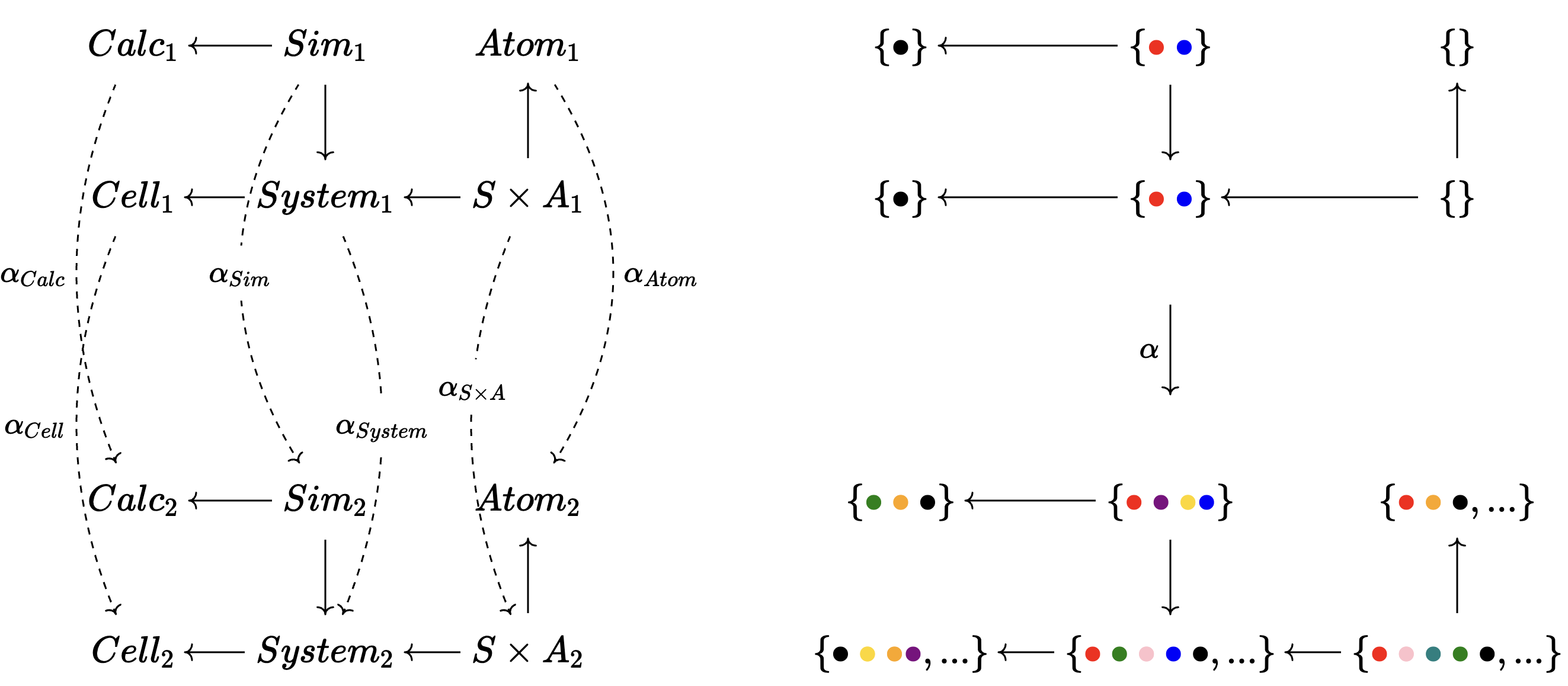
🗄️. Data migration

\[\overset{\Sigma}\Rightarrow\]

\[\longrightarrow\]

\[\underset{\Delta}\Leftarrow\]

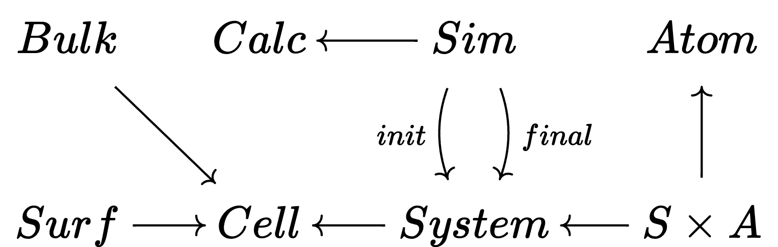
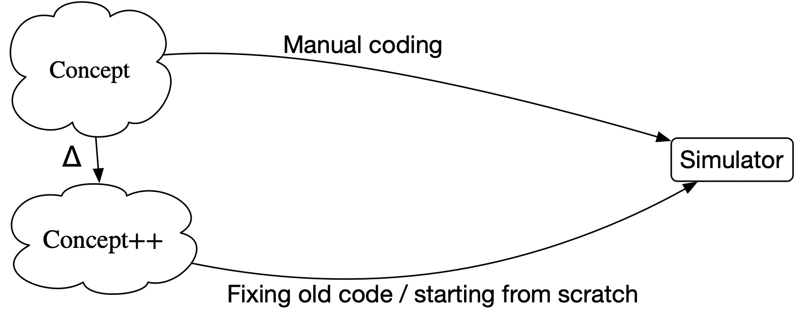
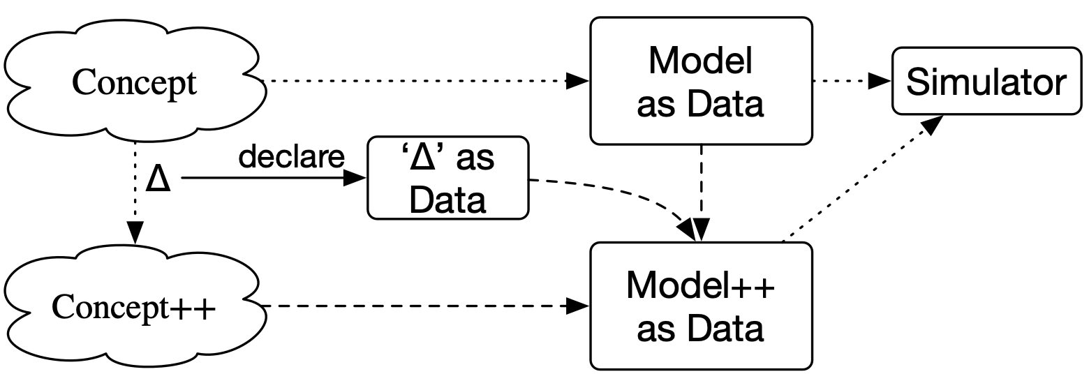
• When you design a schema to contain your data, you will soon learn it needs to be updated. This is a huge problem.

• Schemas are actually categories; functors between them automatically induce data migrations on arbitrary databases.

• When your algorithm is expressed in terms of ACSets, then you can migrate your algorithm automatically, too!

The last thing I’ll talk about in this section is a really powerful technique called Data Migration. This is important because we’ll inevitably discover we want to change our schema as we start using it more and learn more about the world.

On the left is our old schema, on the right is version 2, where we distinguish bulk and surface cells as well as distinguish the input system of a simulation and the final result of optimization. There is something called a functor which we can declare to explicitly relate the two schemas, it amounts to saying for each object on the left which object on the right it relates to and likewise for the arrows. Given this data, the math tells us how to automatically perform data migration on actual concrete databases.

Data migrations preserve information in predictable ways. Sigma migrations move data forward along the functor, and delta migration moves data backwards.

🗄️. Data migration

\[\overset{\Sigma}\Rightarrow\]

\[\longrightarrow\]

\[\underset{\Delta}\Leftarrow\]

# Python
"""System we know nothing about (except pbc)"""
def unknown(pbc):
  if pbc == [True,True,True]:
    return System(Bulk(0,0,0,pbc), [])
  else if pbc == [True, True, False]:
    return System(Surf(0,0,0,pbc), [])
"""Migrate a Sim to a Sim2"""
def migrate_sim(sim::Sim):
  init_sys = System2(sim.cell, sim.atoms)
  final_sys = unknown(init_sys.cell.pbc)
  return Sim2(sim.calc, init_sys, final_sys)

for old_sim in get_sims(old_db_cxn):
  insert_sim(migrate_sim(old_sim), new_db_cxn)

new_query = "SELECT S1.pth, S2.pth FROM ..."

# AlgebraicJulia
"""Declare relationship between schemas"""
F = FinFunctor((system=final,), Simulations, NewSimulations)

"""Constraints"""
Bb, Sb = [true,true,true], [true,true,false]
B = @acset_colim Sims begin b::Bulk; pbc(cell(b))==Bb end
S = @acset_colim Sims begin s::Surf; pbc(cell(b))==Sb end
CB = @acset Sims begin Cell=1; pbc=Bb end
CS = @acset Sims begin Cell=1; pbc=Sb end
constraints = [homomorphism(CB,B), homomorphism(CS,S)]

# Migrate old data
new_simulation_db = Σ(F,constraints)(sims)

# Migrate old query, Q
new_Q = Σ(F,constraints)(Q)

So now our scenario is to update our old data and our query from before into the new schema. I want you to remember that figure I had in the beginning that was contrasting with the status quo. The status quo begins with a conceptual idea, and then we do some manual code implementation that hopefully reflects that idea. So I have some idea how to manually convert a Simulation#1 into a Simulation#2. I know it has the same calculator, that the initial system#2 is the same as the old simulation’s system, and that I don’t know anything about the final other than its cell.

So we manually implement this code which we think is faithful to that conceptual understanding (I tried to write it correctly but turns out it has mistakes, oops), and we leave no formal record of that conceptual idea.

On the right we make the conceptual idea explicit. The only nontrivial data is to say where system goes: init or final? Here the domain expert really has to make a choice, and this is a good illustration how what we’re doing is not black box magic - everything in this talk is something that is rigorously and explicitly expressed by the domain expert; it just happens to be actually usable because we’re working at the level of conceptual abstraction that the domain expert is already thinking at.

So we declare this realtionship between the schemas, and there is also a way of communicating how the periodic boundary condition of the cell indiciates whether or not it is a bulk or surface cell (here a homomorphism is playing the role of declaring this constraint, “If you have a cell with all periodic boundary conditions then it is a bulk cell”, as another example of its versatility). Because we understand these ideas mathematically, we do not have to write any further code to do the migration. We get the further benefit that our queries can now be migrated, whereas on the left we have to write new SQL query to answer the old question.

🗄️. Takeaways

• Filesystem \(<\) Classes
  • More flexible data model than mere tree structure
  • Can write modular code for different components of data model

• Classes \(<\) Database
  • Abstract away the tedium of designing efficient storage for each new structure
  • Uniform language for querying the data

• Database \(<\) ACSet
  • Many schema-agnostic algorithms
  • Automated data migration tools

In each case, the fragility of the code you write decreases.

So to review: when we move from a filesystem to custom datatypes in your programming language, we make the structure of our data explicit and avoid the assumption of a tree structure.

. . .

When we move to the database picture, we no longer have to worry about efficient storage and retrieval of information, and our language for querying the data stays the same when the schema changes. However, to do things other than querying the data, we need to regress back to the class-based approach, and that means that code is extremely fragile to changes in our schema.

. . .

When we view databases category theoretically, as ACSets, we can automatically update our queries to changes of schema and we can do much more things than querying in a way that is uniform with respect to our choice of data structure. Examples of that will be throughout the rest of the talk.

The takeaway message is that, in each case, our data fragility was reduced.

Outline

1. 🗄️ Data
   • CT: C-Sets, Homomorphisms, Data migration
   • Examples: Computational chemistry simulation generated data

2. 💭 Models
   • CT: Colimits, Limits
   • Examples: COVID models, Chemical Reaction Networks

3. 📈 Simulation
   • CT: Functors, DWDs, rewriting
   • Examples: Multiphysics PDEs, Agent-based models

💭 Models through the eyes of the computer

A COVID-19 model. At least in this format, it’s utterly unintelligible, but there’s actually a lot of rich structure that is hidden because it lives in the minds of the researchers who made this. In this section I’m going to argue that two central CT abstractions, called limits and colimits, when considered in the category of chemical reaction networks, correspond precisely to the scientist’s mental model which allows them to informationally compress this thing down to something intelligible.

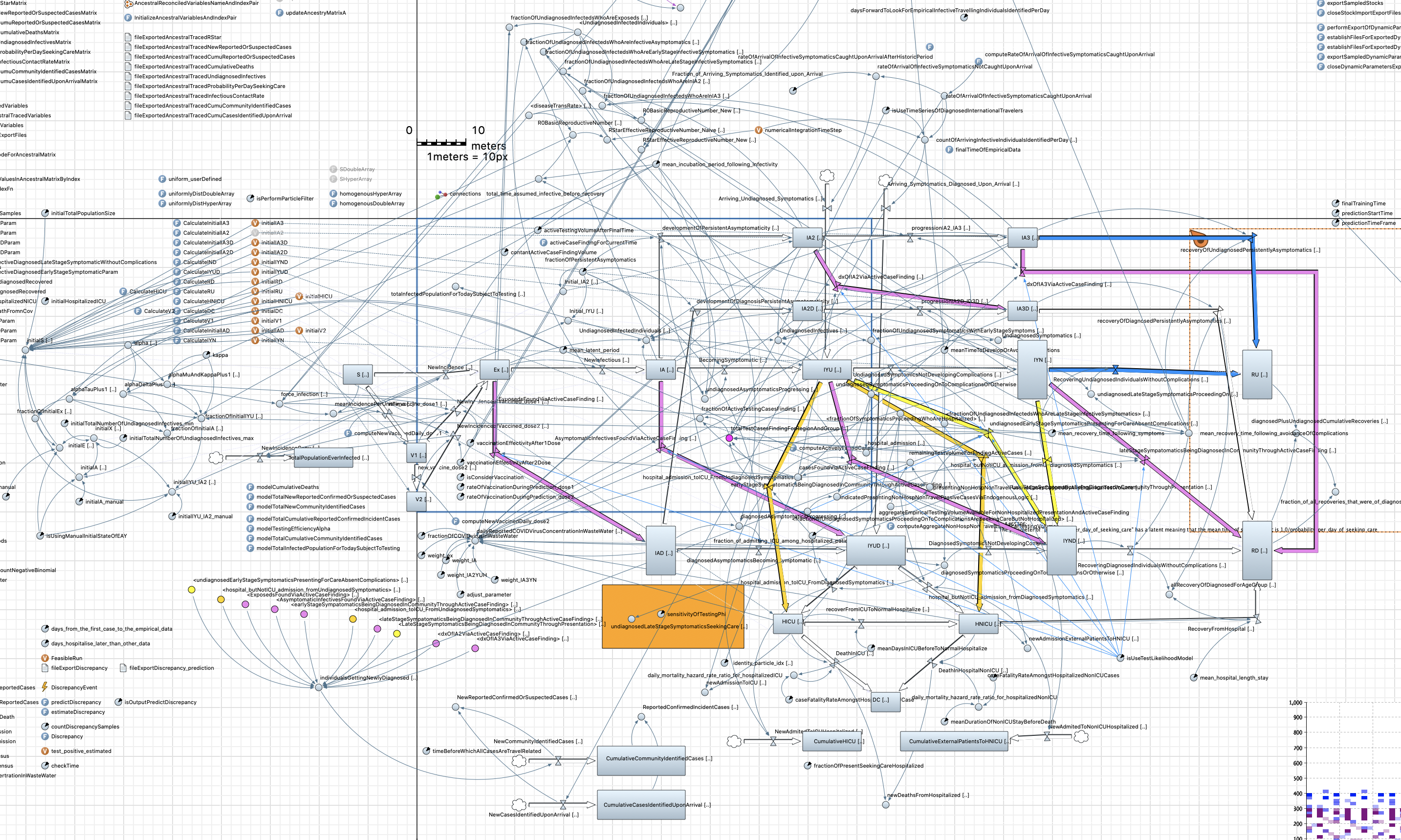
💭 Models through the eyes of the scientist

This might be what a compressed version of the above model which shows how there are different conceptual models being combined. There are three main components, a disease model a demographic model and a spatial model, and all of these submodels are combined via either something addition-like or multiplication-like, in a way that we’ll make precise in this section of the talk.

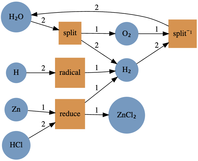
💭 C-Set for Chemical Reaction Networks

The category of Petri nets are just \(\mathsf{C}\)-Sets for a specific \(\mathsf{C}\).

\[2\text{H}_2\text{O}\leftrightarrows 2\text{H}_2+\text{O}_2\]

\[2\text{H}\rightarrow \text{H}_2\]

\[\text{Zn}+2\text{HCl}\rightarrow \text{ZnCl}_2+\text{H}_2\]

using AlgebraicPetri
crn = LabelledPetriNet(
 [:H₂O, :H₂, :O₂, :H, :Zn, :ZnCl₂, :HCl],
 :split   =>((:H₂O, :H₂O)=>(:H₂, :H₂, :O₂)),
 :split⁻¹ =>((:H₂, :H₂, :O₂)=>(:H₂O, :H₂O)),
 :radical =>((:H,:H)=>:H₂),
 :reduce  =>((:Zn,:HCl,:HCl)=>(:ZnCl₂,:H₂)),
)

┌───┬─────────┐
│ T │   tname │
├───┼─────────┤
│ 1 │   split │
│ 2 │ split⁻¹ │
│ 3 │ radical │
│ 4 │  reduce │
└───┴─────────┘
┌───┬───────┐
│ S │ sname │
├───┼───────┤
│ 1 │   H₂O │
│ 2 │    H₂ │
│ 3 │    O₂ │
│ 4 │     H │
│...│   ... │
└───┴───────┘
3 rows omitted

┌───┬───┬───┐
│ I │it │is │
├───┼───┼───┤
│ 1 │ 1 │ 1 │
│ 2 │ 1 │ 1 │
│ 3 │ 2 │ 2 │
│ 4 │ 2 │ 2 │
│...│...│...│
└───┴───┴───┘
  6 rows omitted
┌───┬───┬───┐
│ O │ot │os │
├───┼───┼───┤
│ 1 │ 1 │ 2 │
│ 2 │ 1 │ 2 │
│ 3 │ 1 │ 3 │
│ 4 │ 2 │ 1 │
│...│...│...│
└───┴───┴───┘
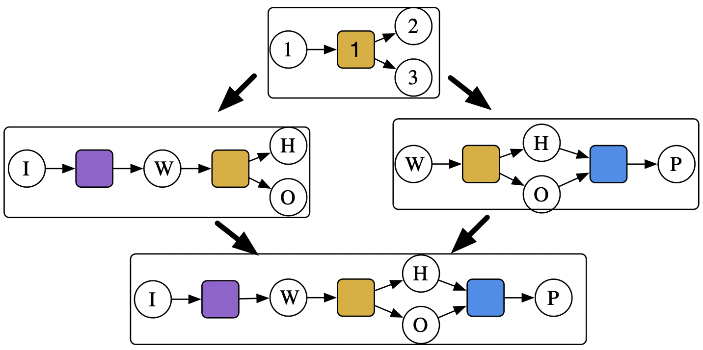
 4 rows omitted

Luckily I don’t need to tell you something new to teach you how we represent chemical reaction networks, since I’ve already introduce C-sets. It turns out we can pick a particular schema and capture the data perfectly well. … There are four objects and four arrows. Think of \(S\) and \(T\) as different kinds of vertices in a directed graph, called species and transitions. Think of \(I\) and \(O\) as two kinds of arrows, those that point from \(S\) to \(T\) and those that point from \(T\) to \(S\).

With Algebraic Petri, which is a library in AlgebraicJulia which focuses on this particular kind of C-Set, we declare it with this syntax and can view the result as a database or as a visualization. This representation is called Petri Net where the square nodes are reactions and the circular nodes are species.

💭 Colimits of CSets: gluing models together

# Python
class Species():
 def __init__(self, name: str):
class State():
 def __init__(self, species: Dict[Species, Int]):
class Rxn():
 def __init__(self, name: str, i: State, o: State):
class RxnNet():
 def __init__(self, rxns: List[Rxn]):

# AlgebraicJulia
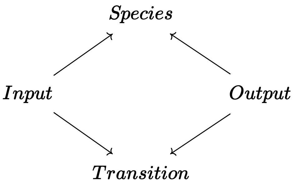
@present LabeledPetriNet(FreeSchema) begin
  (S, T, I, O)::Ob
  Name::AttrType
  is::Hom(I,S); it::Hom(I,T)
  os::Hom(O,S); ot::Hom(O,T)
  sname::Attr(S,Name)
  tname::Attr(T,Name)
end 

Write a program that combines overlapping reaction networks:

• e.g. \(\boxed{\text{H}_2\text{O}_s\overset{melt}\rightarrow \text{H}_2\text{O}_l\overset{lyse}\rightarrow \text{H}_2+\text{O}_2}\) and \(\boxed{\text{Water}\overset{zap}\rightarrow \text{H gas}+\text{O gas}\overset{oxidize}\rightarrow Peroxide}\)
• This has one overlapping transition and three overlapping species

# Python
def merge(n1:RxnNet, n2:RxnNet,
          s_overlap:list, t_overlap:list):
  n1_rxn = deepcopy(n1.rxns)
  for r2 in n2.rxns:
    n_pairs = [(r1.name,r2.name) for r1 in n1_rxn]
    if not intersect(t_overlap, n_pairs):
      n1_rxn.append(rename_state(r2, s_overlap))
  return RxnNet(n1_rxn)

def rename_state(r::Rxn, s_overlap):
  s_dict = dict([(v,k) for (k,v) in s_overlap])
  Rxn(r.name, rename_species(r.i, s_dict), 
              rename_species(r.o, s_dict))

def rename_species(s::Species, s_dict::dict):
  Species(get(s_dict,s.name, s.name))

# AlgebraicJulia
overlap = @acset PetriNet begin 
  S=3; T=1; I=1; O=2; it=1; ot=1; is=1; os=[2,3] 
end 
o_left = homomorphism(overlap, left; monic=true)
o_right = homomorphism(overlap, right; monic=true)
colimit(Span(o_left, o_right)) # standard lib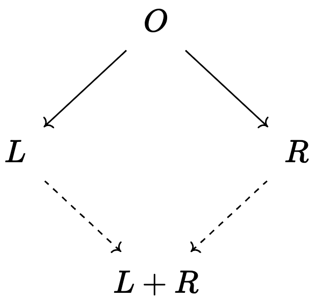

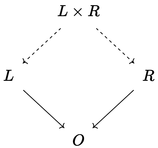
So here is a Python object-oriented representation of the same data to compare against the C-Set version on the right.

. . .

Now our challenge is to write a function which combines two reaction networks along an overlap. For example, here are two which overlap with three different species and one transition.

. . .

The python code is straightforward. We start by taking all of the reactions in rxnet 1. Now it’s just a matter of deciding which of the second rxnet reactions we want to include. So we do some checking of the overlapping names and then make sure to rename species in the reactions that we do include. Do-able, but tedious and unclear if we made mistakes.

On the right hand side, we see a radically different approach. Here the idea is that we need to introduce a third petri net which represents the overlap between our left and right petri nets. This is kind of like how we had a C-set represent the shape of our query before. We provide maps into the Left and the Right to pick out which species and transitions we would like to be merged. Thus the data is a span, i.e. a pair of outward pointing arrows. There is a basic notion in category theory called a “colimit” which, although I won’t be able to explain it in this talk, essentially performs this gluing operation.

So again we’ve just declared our concept explicitly rather than implementing it, thus replacing some ad-hoc code with a clean mathematical idea, and thus we can be sure it is computed correctly and we don’t have to reimplement it for each new data structure: the same code will glue graphs together or databases of simulations.

💭 Limits of CSets: model multiplication

Write a program that multiplies all stoichiometry by 2:

# Python
def mul2(r: RxnNet):
  RxnNet([Rxn(rxn.name, mul2(rxn.i), mul2(rxn.o))
          for rxn in r.rxns])
def mul2(s: State):
 State(dict([(k,v*2) for (k,v) in s.species.items()]))

# AlgebraicJulia
two = @acset PetriNet begin 
  I=2; O=2; S=1; T=1; 
  is=1; it=1; os=1; ot=1 
end 
mul2(x::PetriNet) = x ⊗ two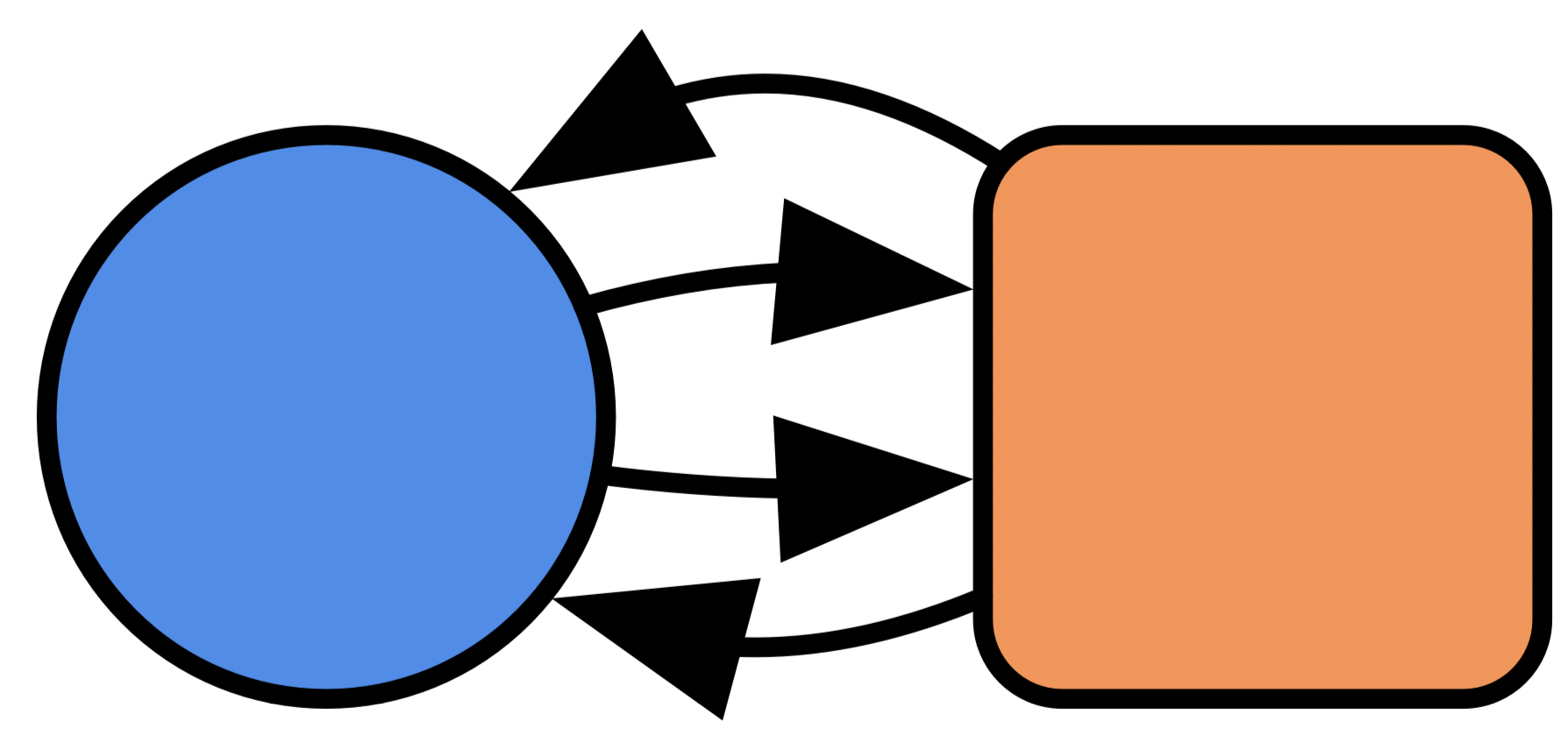 

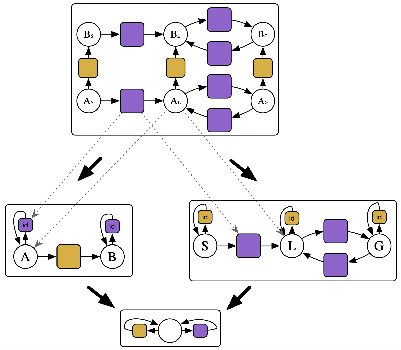
Write a program that stratifies a unary CRN with a CRN of phase transitions:

• e.g. stratifying \(A\rightarrow B\) with \(Solid \rightarrow Liquid \leftrightarrows Gas\) yields:

If colimits are a kind of general notion of addition, limits are a kind of notion of multiplication. For example, suppose we want to multiply the stoichiometry of a reaction network by two? On the left, we have the code you could script up to do this. Yet on the right, we just declare a petri net that is analogous to the number two and take the natural notion of product in the category of petri nets, which is just a built in library function. This does the same thing, which is very cool.

. . .

A more sophisticated kind of model multiplication is called “stratification”. An example of this is taking a chemical reaction network (e.g. A goes to B) and a separate network representing phase transitions (e.g. solid go to liquid, and liquid is in equilibrium with gas), and we apply the phase transitions to both chemical species and we allow the reaction to occur in all three phases. So how are we going to write a function to do this generically?

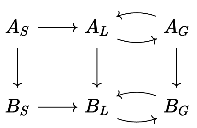
💭 Limits of CSets: model multiplication

Write a program that stratifies a unary CRN with a CRN of phase transitions:

• e.g. stratifying \(A\rightarrow B\) with \(Solid \rightarrow Liquid \leftrightarrows Gas\)

# Python
def strat(r1: RxnNet, r2:RxnNet):
  rs = []
  for rx1 in r1.rxns:
    for s2 in get_states(r2):
      rs.append(rename_rxn(rx1,s2))
  for rx2 in r2.rxns:
    for s1 in get_states(r1):
      rs.append(rename_rxn(rx2,s1))
  return RxnNet(rs)

def rename_rxn(r:Rxn, s: Species):
  return Rxn(r.name, rSt(r.i,s), rSt(r.o,s))

def rSt(st: State, s2:Species)
  return State(Dict([Species(s1.name+s2.name) 
         for (s1,v) in st.species.items()]))
   
def get_states(r::RxnNet):
  ...

To spoil the ending, the AlgebraicJulia approach will be basically the same as as gluing models together, where we just provide the data of two maps and we automatically generate the stratified model.

Well in the python case, we can do two double for loops, where we pair each set of reactions with the other’s set of species. In each of these loops we are going to create a reaction. As always, a specific problem which we can write very specific code in order to solve. The right hand side is interesting. Note that it is completely dual to the diagram I had on the previous side for colimits; we’re just reversing the arrows. So our “overlap” CSet is something that the left and right map into if we are multiplying. It’s amazing that this particular multiplication does the right thing, but there is a catch: the two petri nets we are multiplying aren’t exactly the ones that we were given in the problem statement; they have these “identity transition loops” on each object.

We could write some ad hoc code in Julia to manually add these loops and manually construct the functions into the overlap C-Set, but on the next slide I’ll show there’s a cleaner way to do this.

💭 Takeaways

Gluing together models and multiplying models can be made sense of in any category.

• These operations often correspond to our genuine conceptual breakdown of complex systems
  • This is not made explicit in conventional programming.
• These can be efficiently implemented for ACSets/databases generally in a standard library, so that custom code need not be written for each domain.

More than constructing ACSets, there are other things we can do generically, too:

• Applying constraints (blog post)
  • An ACSet morphism is the syntax of constraints
• Quotienting by symmetry (blog post)
  • An ACSet (iso)morphism is a symmetry

In addition to adding and multiplying models, I want to touch upon two other things you can do with models that are not just constructing them in a compositional way. These correspond to two blog posts I’ve made on the algebraicjulia blog.

Outline

1. 🗄️ Data
   • CT: C-Sets, Homomorphisms, Data migration
   • Examples: Computational chemistry simulation generated data
2. 💭 Models
   • CT: Colimits, Limits
   • Examples: COVID models, Chemical Reaction Networks

3. 📈 Simulation
   • CT: Functors, DWDs, rewriting
   • Examples: Multiphysics PDEs, Agent-based models

📈 Continuous time simulations

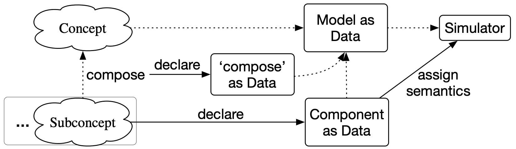
Simulations shouldn’t be written as code. The model should be compiled to simulation.

Code is a good semantics category, but lousy for syntax (can’t do fancy things like limits and colimits in it).

Advection-Diffusion Equation Solver in Python

# Python
def F(rho, v, MeshCoordi,facenodes,centroid): # advection flux coeff
    return -rho*(v @ fnormal(MeshCoordi,facenodes,centroid))

def get_linMatrix(pymesh, custom_mesh, dt, phi0):
  . . . 
  totalMeshCells=len(MeshCells)
  fluxMat=numpy.zeros((totalMeshCells, totalMeshCells))
  bMat=numpy.zeros((totalMeshCells,1))
  for c_cell in range(totalMeshCells):
    n_index=0
    for n_cell in neighbourID[c_cell]: #n_cell neighbouring cell index
      c_ni_faceNodes=cellFaceID[commonFace[c_cell,n_index]]
      if n_cell == None:  #this will handle the boundary cell elements
        fluxMat[c_cell,c_cell], bMat[c_cell]=get_Bcondition(...)
      else: #non boundary elements
        #D is diffusion flux contribution
        D=gamma*gDiff(MeshCoordi,c_ni_faceNodes,[...])
        #A is advection flux contribution
        A=F(rho,numpy.array([ux,uy]),MeshCoordi,c_ni_faceNodes,[...])
        fluxMat[c_cell,n_cell]=-(D*funA(A,D) + max(A,0)) #General scheme by Patankar 
      n_index+=1

    bMat[c_cell]+=rho*cellvolume[c_cell]*phi0[c_cell]/dt
    fluxMat[c_cell,c_cell]+= -( numpy.sum(fluxMat[c_cell,:]) - fluxMat[c_cell,c_cell] ) + rho*cellvolume[c_cell]/dt
  return fluxMat, bMat

Conceptual model:

Problem

Implementation details to worry about when we update the math

• how much does order matter?
• which for loops need modification?
• which parts are geometry vs physics?

Extending what I’ve said so far to the design of simulators amounts to the following:

• simulations should be compiled to code rather than written in code
• This is because we can do high level conceptual programming (e.g. limits and colimits) when we are working with data, whereas representing our simulation via code will forever condemn us to having every conceptual update require a painstaking manual code update that could be very challenging.

For example, the code here I took from a github repo that scopes out computing advection and diffusion physics, captured by that equation on the right, exemplifies the disconnect between the mathematical model and the implementation.

When we work at this low level, introducing a simple mathematical idea (for example adding a gravitation force) forces us to remind ourself of all the implementation details - there could be a cascade of changes required.

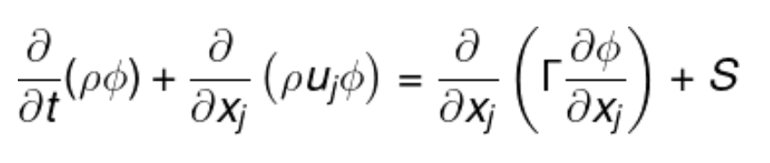
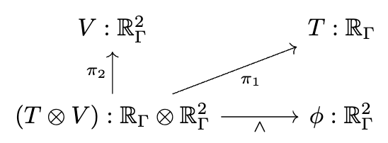
📈 Multiphysics modeling

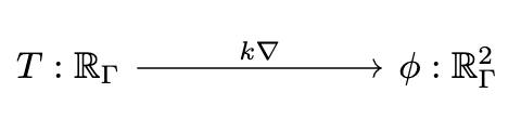
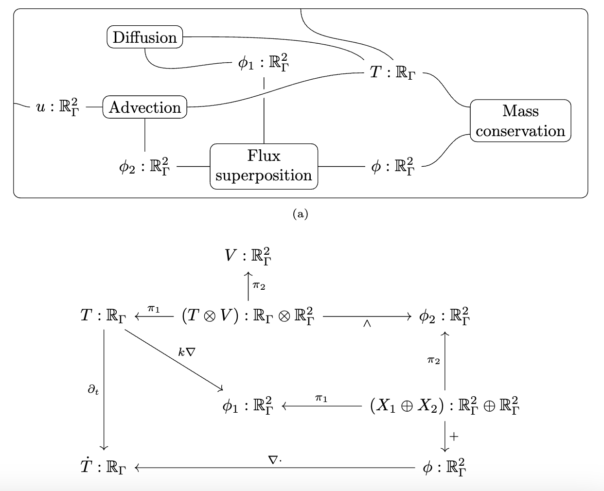
# AlgebraicJulia
"""Define the multiphysics"""
Diffusion = @decapode DiffusionQuantities begin
  C::Form0{X}
  ϕ::Form1{X}
  ϕ == k(d₀{X}(C))   # Fick's first law
end
Advection = @decapode DiffusionQuantities begin
  C::Form0{X}
  (V, ϕ)::Form1{X}
  ϕ == ∧₀₁{X}(C,V)
end
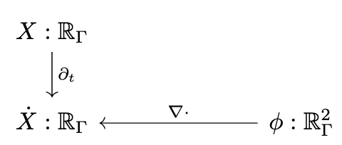
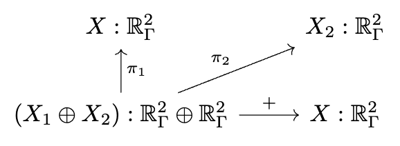
Superposition = @decapode DiffusionQuantities begin
  (C, Ċ)::Form0{X}
  (ϕ, ϕ₁, ϕ₂)::Form1{X}
  ϕ == ϕ₁ + ϕ₂
  Ċ == ⋆₀⁻¹{X}(dual_d₁{X}(⋆₁{X}(ϕ)))
  ∂ₜ{Form0{X}}(C) == Ċ
end
compose_diff_adv = @relation (C, V) begin
  diffusion(C, ϕ₁)
  advection(C, ϕ₂, V)
  superposition(ϕ₁, ϕ₂, ϕ, C)
end

"""Geometry"""
mesh = loadmesh(Torus_30x10()) 

"""Assign semantics to operators"""
funcs = sym2func(mesh)
funcs[:k] = Dict(:operator => 0.05 * I(ne(mesh)), 
  :type => MatrixFunc())
funcs[:⋆₁] = Dict(:operator => ⋆(Val{1}, mesh, 
  hodge=DiagonalHodge()), :type => MatrixFunc());
funcs[:∧₀₁] = Dict(:operator => (r, c,v)->r .= 
  ∧(Tuple{0,1}, mesh, c, v), :type => InPlaceFunc())

I can only briefly gesture at the work done by some of my colleagues in a compositional language for multiphysics. The idea is that there is a graphical language for specifying equations which rigorously corresponds to things like Fick’s law of diffusion and conservation of mass. This is just like how our Petri Nets were a nice graphical language which could rigorously be interpreted as Chemical Reaction Networks and how spans of models can be rigorously interpreted as models glued along an overlap.

There is some interesting math behind how this works which I won’t be able to get into, involving something called the “discrete exterior calculus”, but from a user perspective you can see us declaring each of these small diagrams and then composing them together along shared variables into a multi-physics. We then need to give a computational semantics by associating linear operators with some of the primitive building blocks, such as “multiplication by k” being 0.05 times the identity matrix.

We decoupled the high level physics from the geometry and the implementation.

📈 Continuous time simulation

The result of the simulation is here. We can add in new physics on the fly. You can’t do that with COMSOL.

📈 Agent based models

# Python
class Wolf():
  def init(self, eng: int, position):
  def move(self):
    ...
class Sheep():
  def init(self, eng: int, position):
  def move(self):
    ...
class Grass():
  def init(self, eng: int, position):
  def increment(self):
    ...
class Graph():
  def init(self, vertices, edges):
class World():
  def init(self, graph, ws: list[Wolf], ss: list[Sheep]):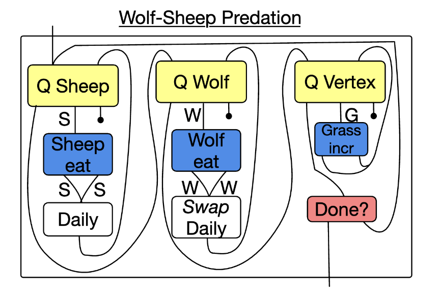

def run_simulation(NSTEPS: int, world: World):
  for t in range(NSTEPS):
    for w in world.wolves:
      w.move()
      w.turn()
      w.eat()
      w.reproduce()
      w.starve()
    for s in world.sheep:
      s.move()
      s.turn()
      s.eat()
      s.reproduce()
      s.starve()
    for g in world.grass:
      g.increment()
    if length(world.wolves) == 0:
      break

# AlgebraicJulia
Pat = @acset_colim WS begin 
  s::Sheep; w::Wolf; sheep_loc(s)==wolf_loc(w) 
end
Repl = @acset_colim WS begin w::Wolf end

wolf_eat = Rule(homomorphism(Pat, Repl), id(Repl);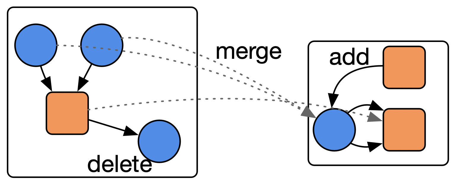 
                expr=(Eng=Dict(1=>vs->vs[3]+vs[2],)))

Now lets imagine performing a discrete time simulation, where there are agents who every time step have some set of actions that they do that interact with an environment.

On the left, we have the standard way we would use code to write a simulation, but this is hiding the structure of our knowledge of the model within code, rather than representing it directly as data. As a consequence of that, when we want to update an assumption, such as changing the terrain the wolves and sheep live on from a grid to an arbitrary graph, the code cannot be automatically updated. Furthermore, there are certain symmetries at a high level between what wolves and sheep do (basically, everything except the way they eat). This high level operation can be made explicit in the AlgebraicJulia code, whereas we can’t straightforwardly derive the sheep code as a function of what we wrote down for the wolf code.

On the right, we see how we’ve compose a bunch of sub-procedures into an overall simulation. An example rewrite rule is shown, where a wolf eats a sheep and acquires its energy if they’re on the same vertex.

📈 Merging, deleting, copying, adding … without code

Task: find a reaction \(A + B \rightarrow C\), delete \(C\) from the reaction network (if no other reactions need it), merge \(A\) and \(B\) together into \(AB\), and add a reaction \(\varnothing \rightarrow AB\)

# Python
def merge_delete_add(r:RxnNet):
  # try to rewrite each reaction 
  for (i,rxn) in enumerate(r.rxns):
    # determine if has at least two inputs
    if sum(rxn.i.species.values()) < 2:
      continue # cannot rewrite this rxn
    # determine if we can delete an output
    C = None 
    for out_species in rxn.o.species.keys():
      appears_in = [j for (j, jrxn) in enumerate(r.rxns)
         if out_species not in (jrxn.i.species 
          | jrxn.o.species)]
      if appears_in == [i]:
        C = out_species 
    if C is not None: # we can delete an output
      out_state = State(Dict([(k,v-1 if k == C else v) 
                    for k,v in rxn.o.species.items()]))
      # . . . etc.
      # to do: merge two input states
      # to do: add a rxn that creates that merged state

• What if pattern was changed?
• What if more than one reaction?
• What if reactions merged?

# AlgebraicJulia
Pattern = @acset PetriNet begin 
  S=3; T=1; I=2; O=1; it=1; ot=1; is=[1,2]; os=[3] 
end

# Subobject of Pattern which we do not delete
I = @acset PetriNet begin S=2;T=1;I=2;it=1;is=[1,2];end

Replacement = @acset PetriNet begin 
  S=1; T=2; I=2; O=1; it=1; ot=2; is=1; os=1 
end

rule = Rule(homomorphism(I,Pattern), 
            homomorphism(I,Replacement))
rewrite(rule, my_rxnet) # uses colimits underneath!

Merging, deleting, copying, adding data … these are all things that you’d first thing require us to stop with the cute pictures and start writing some real good old-fashioned code. However I want to argue this isn’t the case. Let’s return to Petri Nets. Starting from some reaction network, suppose we want to find some reaction that combines two things and delete the result (but we can’t do this if any other reaction makes reference to that result). We also want to have this operation we perform make A equal to B (for example, forgetting the difference between a hydrogen and deuterium atom), and furthermore we want to add a reaction which just produce this AB-hybrid from nothing. That’s clearly a contrived example but I just wanted to show off all of these things in a single example.

So how would we approach this with Python… it’s very hard to write. Even just to find a C that can be deleted, I gave up before we actually merging and adding. Now we have to ask how this changes if the pattern were changed or there were more than one reaction, and all this code breaks. I had tried to make my job easier by making certain assumptions to based on doing this specific rewrite.

On the other side we basically have to draw two pictures, the pattern we are seeking (which is itself a Petri Net) and the pattern we are replacing with, and a relation between them. We declare that data in terms of a Petri nets and their morphisms and simply call rewrite to get the desired result. As a fun fact, underneath the hood this is using colimit infrastructure I talked about in the previous section, as evidence of colimits being a good abstraction.

Conclusions

Lack of automation due to unclear context and assumptions: models are not explicit.

Formalization creates possibility of automation - important as science scales both in amount of data and conceptual complexity of the data.

So to conclude let me bring back these diagrams from the start of the talk. I hope I’ve shown lots of examples of how this paradigm contrasts from the status quo. I hope to have shown that we can make our models and their changes more explicit, and thus avoid “low level” scripting. This explicitness and high-level interaction with computers is essential to doing things automatically and at scale.

Conclusions

CT is useful for the same reason interfaces are generally useful. In particular, CT provides generalized notions of

• multiplication / multidimensionality
• adding things side-by-side
• gluing things along a common boundary
• looking for a pattern
• find-and-replace a pattern
• parallel vs sequential processes

• Mad Libs style filling in of wildcards
• Zero and One
• A point
• “Open” systems
• Subsystems
• Enforcing equations
• Symmetry

These abstractions all fit very nicely with each other:

• conceptually built out of basic ideas of limits, colimits, and morphisms.

We can use them to replace a large amount of our code with high level, conceptual data.

I hope to have shown that just a few basic concepts in category theory, in particular morphisms, limits, and colimits, are a very versatile vocabulary of good abstractions. Various combinations of these are sufficient to capture all of the diverse kinds of activities you see up here in a very generic way that can be specialized to your domain once you view it categorically.

Resources

• Papers and talks: algebraicjulia.org
  • Computational chemistry database integration
  • Epidemiology and gene regulatory networks
  • Chemical reaction network model space exploration
• Blog posts: algebraicjulia.org/blog and topos.site/blog
  • Introductory posts on C-Sets
  • What is a scientific model?
  • Building dynamical systems compositionally
• Code: github.com/AlgebraicJulia
  • DECAPODES.jl
  • AlgebraicPetri.jl
  • AlgebraicRewriting.jl
• For software engineers: Blog post
• This talk: krisb.org/research#talks

If you want to follow up on any the ideas in this talk, we have lots of papers, a couple of which I point out here to be potentially of interest to scientists. We also write blog posts intended to be more accessible and conversational, and I highlight a few here. Our code is always open source and we’re delighted to see it getting used. Lastly the talk itself is available online on my website, in case you want to click on links or see things in more detail (You can also see my extensive speaker notes there).

Backup slides

🗄️. Why not structured?

Why don’t researchers often don’t make structure of data explicit?

Difficult to reap the benefits of structure

The data when sitting still may be structured, but the moment you have to do something with it, you have to load from the database back into ad hoc data structures and code.

• e.g. I want to do a kinetics simulation based on the data within the database

Difficult to maintain the structure

Structure codifies certain assumptions made - when those assumptions change, it can be a lot of work to make things right again.

• e.g. we assumed we were only working with orthorhombic crystal structures, things that touch the Cell class break once we go hexagonal.

So given that databases address this important problem of generic + efficient storage of data and querying, why aren’t they more widespread in science? I think there are at least two technical reasons:

1. There’s basically one thing you do with databases, which is query them. All the rest of our modeling, simulation, and analysis pipeline will have to directly deal with the results of queries, which means your code will have to change when your schema changes.

2. The second point is that a scientist’s model of the world is likely to change somewhat frequently. It’s very tedious to automatically update all of your old data and queries and analysis scripts that use the data.

💭 Generic model stratification

"""Each S has a distinguished reflexive I, O, T"""
@present SchReflPetriNet <: PetriNet begin 
  refl_i::Hom(S,I)
  refl_o::Hom(S,O)
  refl_i ⋅ is == id
  refl_o ⋅ os == id
  refl_i ⋅ it == refl_o ⋅ ot
end

F = FinFunctor(SchPetriNet, SchReflPetriNet)

base = @acset PetriNet begin
  S=1; T=2; I=2; O=2;
  is=1; os=1; it=[1,2]; ot=[1,2] 
end

"""
Apply Σ;Δ migration to input X, then map into base
X transitions are sent to 1, added refl transitions to 2 
(vice-versa if t = false)
"""
function strat_arr(X::PetriNet, t::Bool)
  to_refl = ΣΔ(F)(X) # yields a morphism X → X′
  Refl = codom(X_X′) # X, with reflective transitions
  L = collect(to_refl[:T]) # set of original T's in X

  # Determine where to send transitions in base
  t_init = [p ∈ L ? t : !t for p in parts(Refl,:T)] .+ 1

  homomorphism(Refl, base; initial=(T=t_init,))
end 

function stratify(X::PetriNet, Y::PetriNet) 
  csp = Cospan(strat_arr(X, true), strat_arr(Y, false))
  return Limit(csp)
end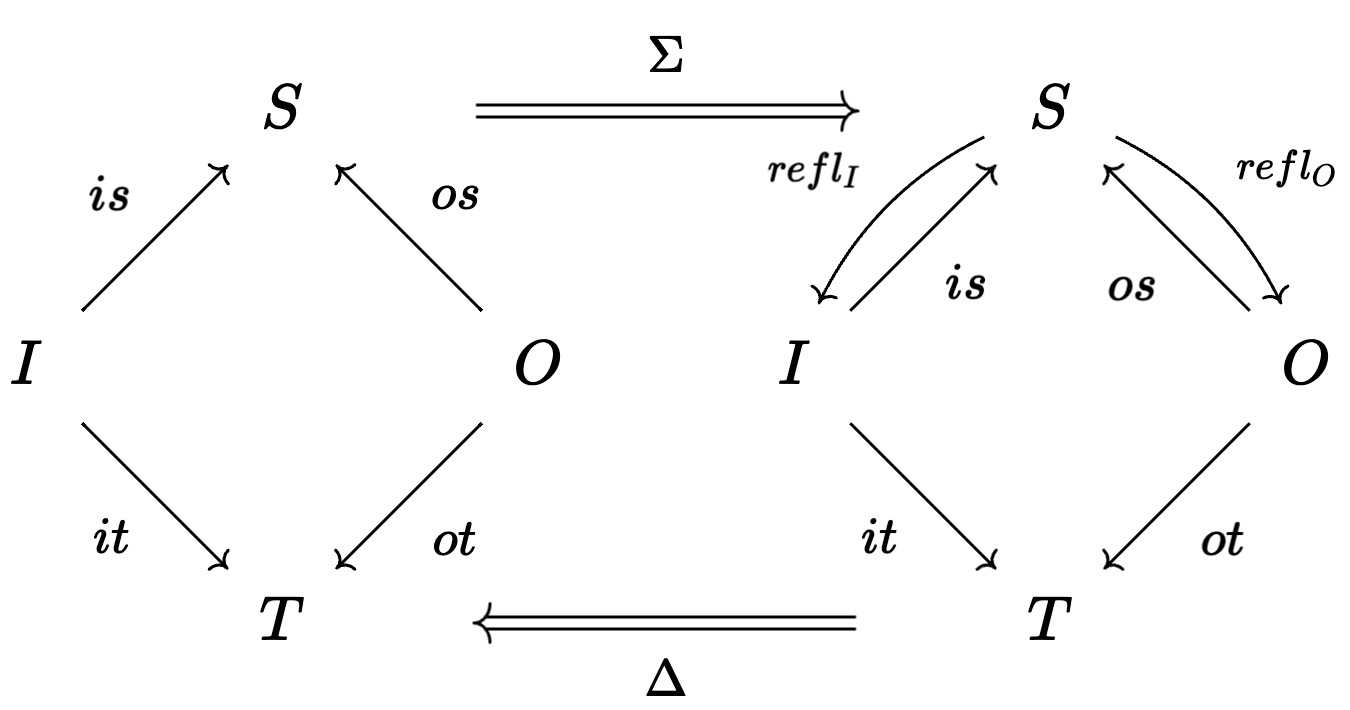 

Given our starting materials, how do we construct the corresponding Petri nets and morphisms into the base Petri net? In this case, we need to recognize that our input Petri nets wish they were living in this other database schema, which I’ll call a Reflexive Petri Net. In that schema, each species has a designated Input/Output/Transition which satisfies the reflexive property. There is a natural way to relate the Petri net schema to the Reflexive one, so we can do a sigma data migration to take an arbitrary Petri net and create one with reflexive transitions. However, what we want is just an ordinary Petri net, so we can immediately apply a delta data migration and get what we need. These data migrations retain enough information to tell us which of the transitions in our result were the original transitions and which were the ones that got automatically added, and we use this information to create the two morphisms at the bottom there.

Now that all that setup is done, we simply call Limit and get a construction of our stratified model. Not only do we have the composite model, but we have projection maps which show how each species and transition in the product is related to the original chemical network and the original phase transition network.

Graph morphism

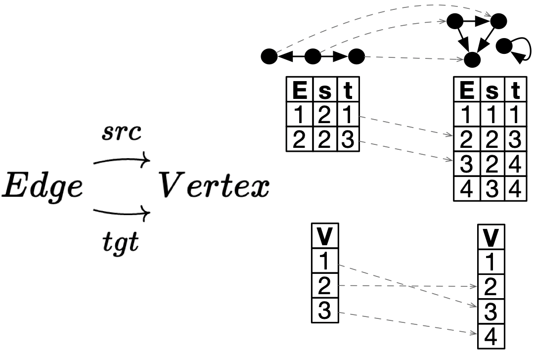
Q = @colim_repr Graph begin 
  (e1, e2)::Edge 
  src(e1) == src(e2)
end
homomorphisms(Q, my_graph)

About Me

Natural science

• 2015, Bachelors at Dartmouth: Physical chemistry / chemical engineering
• 2016, Visiting scholar at EPFL: organometallic synthesis
• 2016-2021, PhD at Stanford (Nørskov group)
  • Applying Density Functional Theory to CO\(_2\) reduction catalysis
  • Developing new DFT functionals for surface modeling

Computer science

• 2019-2020, Google: Software engineering intern
• 2020: Rotation in formal verification (Barrett Group)

Math + CS + Natural science

• 2022, UF: Postdoc in applied category theory (Fairbanks Group)
• 2023, Topos Institute: researcher, AlgebraicJulia developer

My background was first in wet lab chemistry, and I moved into computational science where it seemed like things would be cleaner. However, I soon developed feeling of chaos and helplessness. It seemed like people didn’t trust the results from other research groups or even their own colleagues.

There was lots of collaboration and exchange at the human level, but this broke down whenever anyone tried to do something meaningful with data they did not themselves generate because there is so much context and assumptions implicitly baked into the data and the scripts which generated it. (Even if you generated it, it takes a lot of attention to detail to not misuse it.)

. . .

So this led me to interest in how we represent knowledge formally, so that a machine can make sure that conceptually you are dotting your i’s and crossing your t’s when interpreting some code or data. This involved mathematics and computer science which I started learning in parallel. This led to two internships at Google which were research-focused but still had a lot of elements of regular software engineering (which means I learned things like code-review, Git version control). I also did a rotation with another lab, sort of on the side, with a formal verification research group: formal verification is a way of giving a proof that a program does a certain thing, which is way of rigorously representing what a piece of code is supposed to do (as opposed to normal code, where we say what the code is supposed to do in informal documentation, which can only be interpreted by humans).

. . .

I eventually knew enough math and computer science to do an applied math postdoc (in CS) which has transitioned into my current research role at the Topos Institute. I mostly work on a few packages part of AlgebraicJulia, written in the Julia programming language.

Topos is a nonprofit in Berkeley which produces both research papers and open source software that uses category theory to provide accounts of understanding how complex systems function in terms of simpler systems being composed together, and in particular this leads to our scientific modeling team which seeks to represent scientific knowledge likewise in a compositional way.

Misc content

“ACT helps you be more disciplined than you would be with just your intuitions.”

What’s wrong with the semantic web? It seeks a single language to represent everything. C.T. naturally resists this. SW is good at subtype hierarchies, but say you want to model a process - good luck! you might as well be encoding in JSON / XML … the logical framework isn’t helping.

Not a new standard (XKCD) but rather understanding

Why is C.T. pushout special? It helps us generalized beyond graphs

We want to say what the model is. Code is not model. (e.g. Imperial). The model in the scientist’s head may be complex (made up of many components) but it is not complicated (difficult for a human to grasp).

We have a toolbox of abstractions we understand rather than a universal language that can’t be extended once your assumptions change.

Our modeling framework latches onto the domain but we don’t have to start from nothing.